Data driven solution to predictive maintenance

(1)

University of Twente

Behaviour Management and Social Science

Industrial Engineering and Management

Master Thesis

Data driven solution to predictive maintenance

Authors: Xinyi Chen

Supervisors:

Prof. Jos van Hillegersberg Dr. Engin Topan

Supervisors:

Steve Smith CEng MIET Matthew Roberts CEng MIMechE

(2)

Here it comes, another mile stone of life. I will not say this is the end of my student life, as I wish it is not. Learning and exploring has become an essential part of my satisfactory that I can not live without.

Plenty to be grateful for. First of all, for the opportunity provided by my first supervisor Jos van Hillegersberg so that I was able to do my thesis in the UK. Jos was very hard to grab before this project kicked off as he is a very busy person. However, when the thesis officially starts, I can feel how supportive he actually is. I appreciate that Jos is always innovative and ask me to think about more on how to contribute to the academic world not only to practice. His comment is always focus on the content and process and barely on writing(This is also the comment from his other students from BIT and that’s part of the reason I chose him to be my supervisor.) Thus to the reader(fellow student) of this work, if you want your thesis to be done efficiently, you’d better go to him. Secondly, Engin Topan, my second supervisor is able to critically assess my work in technical perspective that influence the way I do the experiment in a more systematical way.

Thirdly I want to thank Tata Steel Shotton and my company supervisors. TATA Steel Shotton is like a family. I have spend a fantastic time here. Both of my supervisors Matthew Roberts and Steve Smith have been given me plenty of trust and freedom. Every report meeting I had was full of en-couragement and complement that drive me to deliver better result every time. I’m also very grateful for the inclusive environment in the company where I get to hangout quite often with colleagues and get to know their families.

Finally, I want to thank my parents to always been supportive to me and have faith in me. My loving boyfriend who has been accompanied me in the UK for 3 months now and has taken up 99% of the housework for me to focus on my work.

Very last word, University of Twente is the very first place that lead me to discover my full potential, to let my work speak for me, to make life long friends and unforgettable memories. I have had a brilliant time there and if I were to be given a second chance I will choose it again.

January 16, 2020 Xinyi

(3)

MANAGEMENT SUMMARY

This project investigates predictive maintenance using data driven methods in the context of indus-tries that are in transition to Industry 4.0. The study is conducted in TATA Steel UK (Shotton) as a case study.

The problem lies in one of the production line called Hot Dip Galvanising Line in TATA Steel Shot-ton. The function of the line is to coat zinc on steel strips to protect the strip surface. The critical part of the Galvanising line is the pot gear which is filled with melted zinc. Three rolls(sink roll, stabilizing roll and correcting roll) are sunk in the zinc pot to carry the strip. The three rolls together are replaced approximately 4 weeks because the bush that is connected to the sink roll is likely to wear out at around 4 weeks. This decision for the maintenance interval is purely based on experience and sometimes the part is overly maintained that when pulling the rolls out the bush hasn’t been worn out. Thus the engineers are keen on getting insights on the wearing pattern of the bush such that the bush can be replaced just in time. Moreover, plenty of data has been logged through sensors in distributed systems but has never been used for decision support, thus the project is aiming at predicting the bush wear with currently available data.

Although the ultimate goal is to improve the maintenance of the pot gear, in this thesis, our goal is only to predict the bush wear and thus the wearing data is the target variable. The wearing data started to be measured during the preparation time of this project at the end of every maintenance cycle when the component is replaced. The wearing data is measured manually by operators. This leads to the first challenge: small sample size due to small size of target variable. By the end of this project 9 samples are available in total.

There are 4 data sources exists for data logging namely: Set up sheet, IBA, EMASS and Data Ware-house. While the target variable is being recorded, all data sources within the company have been investigated to understand the meanings of those data and check the qualities. Intensive literature review has been conducted, aiming to find the vital variables to be used as predictor where massive amount of literature suggests using vibrations as predictor, however, component itself is in a zinc pot, and there were no sensors connected directly to the bush so the vibration data is not available. This is the second challenge faced during the project.

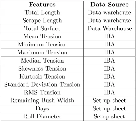
Investigation on metal contact wear was then conducted aiming to find alternative predictors. The Archard’s law is found to be the most common mathematical formula for metal contact wear where sliding distance and force are suggested the two most critical parameters. After investigating into the indicator of sliding distance and force, related variables are extracted from different sources. Time indicator(Number of Days) and environmental indicator(bath temperature) are also extracted for further selection. In the end 14 features are selected as shown in Table 6.7 including the bush wear

(4)

measure. The feature set is selected based on model performance.

Features Data Source Total Length Data warehouse Scrape Length Data warehouse Total Surface Data Warehouse

Mean Tension IBA

Minimum Tension IBA

Maximum Tension IBA

Median Tension IBA

Skewness Tension IBA

Kurtosis Tension IBA

Standard Deviation Tension IBA

RMS Tension IBA

Remaining Bush Width Set up sheet

Days Set up sheet

Roll Diameter Setup sheet

Table 1: Features selected based on PLSR performance

Three modeling techniques that have been used and compared are Partial Least Squared Regression (PLSR), Artificial Neural Network (ANN) and Random Forest (RF). PLSR is chosen because accord-ing to literature it is suitable when the number of independent variables is larger than the sample size and when the dependent variables and independent variables are forming a linear relationship. The linear relation is suggested by literature and by fitting a linear regression to the existing samples we found that the independent variables and the dependent variables did form a linear relation. ANN is selected because it is the most used technique in literature and always produces good results. Some literature suggests that the minimum sample size for ANN is 10. This requirement has not been met yet but will be accomplished in the near future thus ANN is worth investigating. RF is selected be-cause it has also been used in the literature to predict component wear and produces good prediction accuracy. However, both ANN and RF are used when vibrations data are available as predictors in literature.

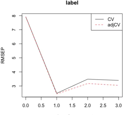
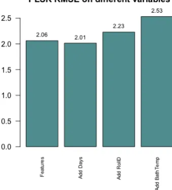
The models are evaluated using cross validation due to small sample size. In order to maximize the training set variance, every time we train the model we use only one sample as test set and the rest as the training set. RMSE is used to evaluate the prediction power of the models and and R squared value are used to see how much variance of the data can the model present. Learning curves are plotted to see how the modeling performance will change when adding more samples to the training set. The result can be found in Table 6.9 and Table 6.10. Learning curve can be found in Figure 6.21 and Figure 6.22. We can see from the result that PLSR is the most suitable model for the current available data. Further more, a monitoring web page has been developed for the engineers to see the bush wearing behaviour online. The web page is based on PLSR model. The user only need to insert the date to see the predicted wearing pattern from the starting date of the corresponding maintenance cycle.

(5)

vari-Data driven solution to predictive maintenance

Training samples PLSR ANN RF

5 2.23 0.39 7.16

6 3.53 4.39 5.65

7 5.74 6.58 6.43

8 4.14 5.26 6.09

Average 3.91 4.15 6.33

Table 2: Modeling RMSE comparison

Training samples PLSR ANN RF

5 0.85 1.00 -0.53

6 0.61 0.40 0.01

7 0.18 -0.07 -0.02

8 0.53 0.25 -0.01

Average 0.55 0.39 -0.14

Table 3: Modeling R2 _comparison

Figure 1: Modeling comparison RMSE Figure 2: Modeling comparisonR2

ables. As a industry in transition period, we discovered challenges when doing predictive maintenance using data driven method. Challenges mainly come from unbalanced and limited samples and the quality issue of data in real life setting.

The limitations are that the current model is built upon a very small sample size thus the model maintenance is critical. The whole modeling process(from feature selection to technique selection) should be conducted repetitively in certain time interval as the performance is subject to change when more data is coming in. The current model is predicting the current wear instead of future wear. Thus the developed web page can be viewed as a monitoring tool instead of a prediction tool. Furthermore, this study has only been looking at the technical perspective of predictive maintenance however there are many other aspects such as economic, regulation and employment etc. All these aspects might bring challenges for implementing predictive maintenance in industries that are in transition period.

(6)

(7)

(8)

1 Introduction 17

1.1 Current Situation . . . 19

1.1.1 Tata Steel Shotton . . . 19

1.1.2 No.6 Hot Dip Galvanising Line . . . 19

1.1.3 Bath gear equipment characteristics . . . 20

1.2 Problem Description . . . 21

1.3 Research Design . . . 22

1.3.1 Research Problem . . . 22

1.3.2 Scope . . . 22

1.3.3 Research questions . . . 22

1.3.4 Method . . . 23

1.3.5 Report structure . . . 24

2 Background Knowledge 26 2.1 Principle component analysis . . . 26

2.2 Artificial Neural Network . . . 27

2.3 Random Forest . . . 28

2.4 Partial Least Squared Regression . . . 28

3 Data collection 29 3.1 Set up sheet . . . 29

3.2 Data warehouse . . . 29

3.3 IBA . . . 30

3.4 EMASS . . . 30

3.5 Data cleaning and integration . . . 30

3.6 Conclusion . . . 31

4 State of Art 32 4.1 Predictive maintenance in industry 4.0 . . . 32

4.2 Mechanical contact wearing behaviour . . . 33

4.3 Data driven methods for wearing prediction . . . 33

4.4 Data pre-possessing . . . 35

4.5 Gaps . . . 36

(9)

Data driven solution to predictive maintenance

5 Data Exploration 39

5.1 Reading Large data sets . . . 39

5.2 Data cleaning . . . 40

5.3 Data prepossessing . . . 40

5.4 Variable selections using PCA . . . 40

5.5 Variables with explanatory power . . . 41

5.6 Unsupervised learning . . . 42

5.6.1 Hierarchical clustering . . . 42

5.6.2 K-means clustering . . . 44

5.6.3 Validation . . . 44

5.7 Correlation and regression . . . 45

6 Modeling and evaluation 49 6.1 Selection of modeling techniques . . . 49

6.2 Feature selection . . . 50

6.3 Data Processing . . . 51

6.4 Partial Least Squared Regression . . . 52

6.4.1 Experiments on extended variables . . . 52

6.4.2 Result interpretation . . . 56

6.5 Neural Network . . . 58

6.5.1 Inner layer and weights tuning . . . 58

6.7 Comparison and evaluation . . . 62

6.8 Discussion . . . 65

6.8.1 Sensitivity to data processing . . . 65

6.8.2 Overfitting . . . 65

6.8.3 Model Evaluation . . . 65

6.8.4 Challenges and Model maintenance . . . 66

6.9 Implementation . . . 67

7 Conclusion and Recommendation (To Practice) 69 7.1 Feasibility . . . 69

7.2 Improvement . . . 69

7.3 Limitation to practice . . . 70

7.4 Implementation . . . 70

7.5 Follow up project development . . . 71

8 Conclusion and Recommendation (To Theory) 73 8.1 Characteristics of industry in transition period . . . 73

8.2 Theory VS Practice . . . 73

8.3 Challenges . . . 74

8.4 Limitation to theory and future research . . . 75

A Data Dictionary 80

B Data exploration plot 86

(10)

C Code 106

C.1 IBA Cleaning Code . . . 106

C.2 EMASS Cleaning Code . . . 111

C.3 Data Visualization and Exploration Code . . . 112

C.4 Modeling code . . . 129

C.5 Tool Development Code . . . 137

(11)

LIST OF FIGURES

1 Modeling comparison RMSE . . . 5

2 Modeling comparison R2 . . . 5

1.1 No.6 Galvanizing line diagram(TATA) . . . 19

1.2 Layout of Bath Gear Equipment Submerged in No.6 Pot(TATA) . . . 20

1.3 Bush(TATA) . . . 21

1.4 Method . . . 24

2.1 Principle component analysis . . . 26

2.2 Artificial Neural Network . . . 27

5.1 Summary Tension . . . 40

5.2 Hierarchical clustering Distance.A2 . . . 42

5.5 K-means clustering on Distance.A2 . . . 44

5.6 K-means clustering on Distance.B3 . . . 44

5.7 Validation for clustering results . . . 45

5.8 linear regression total number of turn, tension std and remaining bush width . . . 45

5.9 linear regression QQ plot . . . 48

6.1 Scaled Modeling data sets . . . 51

6.2 Selection cycle1 as test set . . . 52

6.8 PLSR performance on different feature set . . . 55

6.9 PLSR learning curve on different feature set . . . 55

6.10 Correlation plot cycle1 as test . . . 56

6.16 Neural Network Structure . . . 59

(12)

6.17 RMSE comparison using different test samples to find initial weights . . . 60

6.18 Model performance and selection . . . 60

6.19 ANN learning curve . . . 60

6.20 Learning curve random forest . . . 61

6.21 Modeling comparison RMSE . . . 63

6.22 Modeling comparison R2 . . . 63

6.23 Prediction of 9 samples . . . 64

6.24 Web monitoring page input . . . 67

6.25 Web monitoring page output . . . 67

7.1 Flow diagram . . . 71

8.1 challenges . . . 74

B.1 Mean A2 plot . . . 86

B.2 Minimum A2 plot . . . 86

B.3 Max A2 plot . . . 87

B.4 Kurtosis A2 plot . . . 87

B.5 Skewness A2 plot . . . 87

B.6 Std A2 plot . . . 87

B.7 Median A2 plot . . . 88

B.8 RMS A2 plot . . . 88

B.9 Hcluster A2 plot . . . 88

B.10 K means A2 plot . . . 88

B.11 Principle component A2 plot . . . 89

B.12 PCA A2 plot . . . 89

B.13 Mean A3 plot . . . 89

B.15 Max A3 plot . . . 90

B.18 Std A3 plot . . . 90

B.20 RMS A3 plot . . . 91

B.24 PCA A3 plot . . . 92

B.25 Mean A4 plot . . . 92

B.27 Max A4 plot . . . 93

B.30 Standard deviation A4 plot . . . 93

B.32 RMS A4 plot . . . 94

(13)

B.36 PCA A4 plot . . . 95

B.37 Mean A5 plot . . . 95

B.39 Max A5 plot . . . 96

B.42 Std A5 plot . . . 96

B.44 RMS A5 plot . . . 97

B.48 PCA A5 plot . . . 98

B.49 Mean B3 plot . . . 98

B.50 Minimum B3 plot . . . 98

B.51 Max B3 plot . . . 99

B.52 Kurtosis B3 plot . . . 99

B.53 Skewness B3 plot . . . 99

B.54 Std B3 plot . . . 99

B.55 Median B3 plot . . . 100

B.56 RMS B3 plot . . . 100

B.57 Hcluster B3 plot . . . 100

B.58 K means B3 plot . . . 100

B.59 Principle component B3 plot . . . 101

B.60 PCA B3 plot . . . 101

B.61 Mean B4 plot . . . 101

B.63 Max B4 plot . . . 101

B.66 Std B4 plot . . . 102

B.68 RMS B4 plot . . . 102

B.72 PCA B4 plot . . . 103

B.73 Mean B5 plot . . . 103

B.75 Max B5 plot . . . 103

B.78 Standard deviation B5 plot . . . 104

B.80 RMS B5 plot . . . 104

B.84 PCA B5 plot . . . 105

(14)

(15)

LIST OF TABLES

1 Features selected based on PLSR performance . . . 4

2 Modeling RMSE comparison . . . 5

3 Modeling R2 comparison . . . 5

1.1 Report structure . . . 25

4.1 Survey of essential variables . . . 36

5.1 Variable norms . . . 40

5.2 Variables selected from EMASS . . . 41

5.3 Variables selected from IBA . . . 41

5.4 Created Variables . . . 42

5.5 Explanatory variables correlations with bush wear . . . 46

5.6 Clustering results . . . 48

6.1 Features selected with explanatory power based on the Ardcher’s law . . . 50

6.2 Additional features selected for further experiments . . . 51

6.3 PLSR validation result with standard features(Feature set 1) . . . 54

6.4 PLSR validation result adding ”days”(Feature set2) . . . 54

6.5 Adding ”days” and ”RollD”(Feature set 3) . . . 54

6.6 Adding ”days”,”RollD” and ”Bath Temperature”(Feature set 4) . . . 54

6.7 Features selected based on PLSR performance . . . 58

6.8 Random Forest result validation using LOO . . . 61

6.9 Modeling RMSE comparison . . . 62

6.10 R2 comparison of models . . . 63

6.11 ANN prediction result . . . 63

6.12 PLSR prediction result . . . 64

6.13 RF prediction result . . . 64

A.1 Variables from Data Warehouse . . . 81

A.2 Variables from IBA . . . 83

A.3 Variables from Setup sheet . . . 85

(16)

(17)

CHAPTER

ONE

INTRODUCTION

The latest industrial revolution proposes varieties of smart products such as smart cities and smart grid. While smart industry concept is referred to as ”Industry 4.0”. The concept includes smart manu-facturing, smart factory, lights out manufacturing and internet of things (IOT). (Sniderman 2019) The essential idea of industry 4.0 are automation, connectivity and big data exchange in manufacturing process. Automation leads to not only automotive production but also automotive decision making system. One of the application is predictive maintenance.

Rotating metal to metal contact wear prediction is one of the critical area in predictive maintenance as rotating mechanical components such as bearing and bush are widely implemented in machines and failure of those causes down time of machinery and production line. Existing prognostic methods can be classified into three categories namely are ”Model-based prognostics”, ”Data driven prognos-tic” and ”Reliability-based prognostics” (Tobon-Mejia 2012). Model-based prognostics requires deep knowledge in system functions. Mathematical models are built to represent the system behaviour including component degradation process. However, systems are often complex in reality thus math-ematical modeling is often computationally expensive and assumptions are required when building models. Reliability based prognostics can also be referred to as ”experience-based prognostics” which uses historical data during a significant period of time and discover the statistical distribution for each parameter. Poisson, exponential, weibull and log-normal distribution have been proposed in the literature for failure time distribution. This approach is easy to implement when historical data from significant period of time is available, however, the prediction result is less precise than those with model-based and data driven method. Data driven prognostics aiming at getting information from the raw data mainly from sensors. It uses mainly artificial intelligence tools or statistical models to learn the wearing behaviour and to predict the condition in the future. The model operates automatically without considering the explanatory power to the real system or parameters. Although data driven method is not computational expensive it still provide good prediction results for systems where it is easy to monitor data representing wearing behaviour or system failure. However, critical data such as failure related data are often missing in industry as failure has been prevented in every way possible due to the huge cost of down time (Zschech 2019).

This project conducts a data-driven bush wear prediction based on steel production line in Tata steel Shotton (UK). A critical part of the production line is maintained by replacing the component every four weeks which leads to the fact that there were barely any failures occurred. As the bush operates in melted zinc pot and there is currently no sensors connect to it, the bush remaining width is measured every four weeks thus the wearing data is only available at the end of each maintenance cycle from

(18)

15/05/2019.

The main contributions of this study will be two folds as follows: To academic environment:

-This study provides some characteristics for industries that is in transition to industry 4.0 in terms of predictive maintenance.

-This study finds a possible existing model to use in industry context that was barely used in predictive maintenance before.

-This study discusses the difference between theory and practice and presents challenges could face when doing predictive maintenance and the guidelines to deal with the challenges in industry in tran-sition to industry 4.0.

To practice:

-This study investigates different data source in TATA Steel Shotton reflect on data quality and improvement regarding data logging.

-This study discovers gaps within currently logged data and essential parameters needed for wearing prediction.

-This study gives conclusions on the feasibility of predicting bush wear and prediction results on proposed methods that help TATA steel Shotton gain insight on the big data and the ways to better fit in industry 4.0 concept.

-This study developed a tool to monitor the wear using selected model(s) such that the research result is able to be implemented in operations.

-This study presents business opportunities and following up projects for TATA steel to further improve the current maintenance process as well as expanding the improvement to other sites and other problem area.

(19)

1.1 Current Situation

1.1.1 Tata Steel Shotton

Tata steel shotton is located in Deeside, North Wales, with its annual production of approximately 500,000 tonnes of steel for building envelope, domestic and consumer applications. The plant in Shotton has existed for over 120 years, the colour coated steel products have been produced for over 50 years and are backed by guarantees of up to 40 years. Differentiation has been its strategy with innovative products occupies 75% of the order.(Tata Steel at Shotton fact sheet).There are in total 22 lines in Shotton, the project is based on the No.6 Galvanising line.

1.1.2 No.6 Hot Dip Galvanising Line

Galvanising is the process of coating the steel substrate with zinc to protect the steel from atmospheric contaminants such as water, oxygen and salts such that the steel corrodes slower. The No.6 Galv Line consists of the following sections: Entry, Furnace, Cooling, Bath, After Pot Cooling, Water Quench, Temper Mill, Tension Leveller, Chemical Coater Section, Oiler and Exit Section. These sections are presented in Figure D.2.

Figure 1.1: No.6 Galvanizing line diagram(TATA)

All coils arrive on site by rail and transported on shuttle car from rail head to entry. The raw coils are cropped to remove any off-gauge or damaged steel before being put on entry section. The Furnace section is to clean the strip and prepare it to be suitable for galvanizing. The aim of the cooling section is to reduce strip temperature to about 520°C and stop any further micro-structural changes. There are two bath on No.6 Galv namely Galv Bath and Galfan Bath that galvanize different products. After the strip has passed through the bath, the zinc coating need to be solidified before touching any roll surface. That’s why after pot cooling exist to lower strip temperature to below 280°C. The strip is cooled further in the Water Quench to achieve a strip temperature of 50°C. The Temper mill and tension leveler applies a to the galvanized strip and stretches the strip respectively to improve strip shape, surface finish, mechanical properties and remove yield point elongation.

The Chemical Coater Section applies precisely metered amount of coating to both sides of a moving strip before the Oiler applys a film of oil on one or both sides of the strip. The inspectors can inspect the coil throughout process at the Exit Section. An exit inspection sheet is filled out by exit operators with quality details of the strip. Once the coil has finished it is transported to the packing or storage area for customer or further processing.

(20)

[image:20.595.121.477.126.352.2]

1.1.3 Bath gear equipment characteristics

Figure 1.2: Layout of Bath Gear Equipment Submerged in No.6 Pot(TATA)

The pot gear is a key part of the NO.6 Galvanising Line which consists of three major parts: the sink roll, stabilizing roll and the correcting roll. The layout graph can be found in Figure 1.2. All three rolls are inspected and replaced after 3-4 campaigns(maximum 100 days in bath).

The Sink Roll is always coated with tungsten carbide, the diameter of the sink roll is in between 560mm and 600mm. The roll is connected to standard sleeves that are replaced every Bath cam-paign(4 weeks). Two sets of legs are are connected to sink roll frame that are fitted with concentric bushes. Bushes are replaced after every bath campaign.

Same as the sink roll, the stabilizing roll is tungsten carbide coated as well, with maximum diameter 230mm and minimum diameter 210mm. Roll can be fitted with either standard or coated sleeves based on what is identified on the set up sheets. When the rolls are new from stores they are to be fitted with coated sleeves. The fitted standard sleeves are changed after every bath campaigns. Bearing blocks are fitted with standard length bushes. Blocks are replaced after every campaign and bush can be reused for another campaign.

The correcting rolls has similar characteristics to the stabilizing roll. Only the bearing blocks to be fitted with reduced length bushes except when no reduced length bushes available.

The distance between the correcting roll and stabilizing roll as well as the size of all the rolls in the bath can play an important part in the bow of the strip. Generally it is very hard to produce a flat strip and normally the strip is slightly bowed which causes unbalanced coating on strip.

(21)

in strip and un-stability of the strip increases. Owing to this, the strip is likely to be faulty coated such as non uniformly distributed coating and more dross. The knife shouldn’t be too low to the bath either as it causes splash from the liquid spelter.

1.2 Problem Description

The maintenance cost of the pot gear is increasing drastically during the past years. In 2009, the maintenance cost of pot gear is under £50000 while in 2019 this number has already been increased to£400000. The correcting roll and the sink roll occupies the most of the maintenance cost (TATA).

One of the equipment that is connected to the sink roll is the bush. The bush are replaced after every bath campaign which is expected to be 4 weeks. This is due to the bush wear, by experience, the bush will wear into the legs after 4 weeks. As shown in Figure 1.3, the bush the upper part of the bush is wider than the lower part. According to domain expert, the wearing process is happening to the upper part from the inner circle to the outer circle. When unexpected events happened such as the strip breaks then the bushes also are replaced even if the campaign is not completed. This is an expensive process because every time the bushes are replaced, the whole line has to be shut down, the pot gear is taken out of the bath and replaced with a new set. The old one is inspected, bushes are replaced. Despite the fact that it cost 1507£/hr for the line shut down and it takes 7 hours to replace the pot gear, it is also dangerous assignment for the operators. Thus it is valuable to investigate the cause of the bush wear and potential ways to predict the wearing condition of the bush.

Although plenty of sensors and data loggers are installed in the process and different data storage servers are available, the decisions are still made based on experience. From process point of view, the engineers and the management teams have a brief picture (different prospective) of what may be the reason of the bush wear, however none of those reasons are confirmed or validated. Thus this project has been set up to discover the correlation among different parameters and the relation between a combination of parameters and the bush wear with limited amount of wearing samples. An ideal project out come could be given a set of parameter value in a specific time window, the wearing condition of the bush can be predicted. Such that the operator will only replace the pot gear when it is just necessary and maintenance cost is reduced.

Figure 1.3: Bush(TATA)

(22)

1.3 Research Design

1.3.1 Research Problem

Based on the current situation described in the previous chapter, the goal of this project is to in-vestigate the feasibility of predicting bush wear with current available data and to propose potential methods to predict bush wear using data driven method while wearing data are in small sample size. By gaining insight on the bush condition, the ultimate goal is to prolong maintenance cycle such that maintenance frequency is reduced and so as the maintenance cost. In other words the following question will be answered by the end of this project:

”How can data driven methods be applied to predictive maintenance in industries that are in transition to industry 4.0?”

1.3.2 Scope

This study is mainly looking at data-driven methods to predictive maintenance in terms of predicting the bush wear. Mathematical models may be used to assist on modeling performance but it is not essential. In terms of modeling, artificial intelligence models are used and evaluated. We use bush wear prediction in Tata Steel Shotton as a case representative of predictive maintenance in industries that are in transition to industry 4.0. By solving the specific problem we are likely to be able to reflect on industries in transition period in general.

1.3.3 Research questions

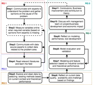
In order to be able to answer the main research question, sub-questions are defined and the corre-sponding approaches of answering each sub questions can be found in Figure 1.4. Steps within the approach are explained in the next section.

Research question 1: What is the current situation in Tata Steel Shotton as an industry that is in transition to industry 4.0?

1a. What is the current maintenance process in Tata Steel Shotton? 1b. What are the existing data that are ready for collection?

1c. What are the meaning of the existing data?

1d. How can the data from different sources be integrated?

Research question 2: How is predictive maintenance fit in industry 4.0 concept and what is the current state of art regarding predictive maintenance using data driven methods?

2a. Which data driven models have been used to predict metal contact wear in industries?

2b. What are the steps that has been used in literature in terms of data prepossessing and model building?

2c. What are the measures to evaluate predictive power of the models?

2d. Based on prediction power and current context which models are the most suitable for predictive maintenance?

2e. What are the gaps and limitations of current literature on predictive maintenance in industry?

Research question 3: How is the quality of industrial data and what are the challenges? 3a. What are the characteristics of industrial data?

(23)

Research question 4: What are the most suitable and feasible machine learning models for wearing prediction in Tata Steel Shotton ?

4a. What features can be extracted from the data set?

4b. What models are suitable to use based on the current available data?

4c. How can the model be trained and how can the modeling performance be evaluated? 4d. How can the predictive model(s) be implemented to the production operation?

Research question 5: What are the business insights that can be extracted from the modeling performance?

5a. Is it feasible to predict the bush condition ?

5b. How can the model performance and current situation regarding data logging and maintenance process be improved based on the findings?

1.3.4 Method

CRISP-DM(Shearer C,2000) has become the most applied and referred approach for data mining expert.(Forbes,2015) However it is a generalized methodology for big data analytic not specifically for predictive analytic. A guideline for predictive analytic has been proposed in (Shmueli & Koppius 2011). During execution of this project, the two methods mentioned above has been combined and modified to fit in real industry context. The detailed steps taken is shown in Figure 1.4

Business understanding and data collection

Step1 to 3 were conducted to answer research question 1a-1d. Meeting were organized to meet line expert and help understand the problem area. It was noticed that different people have their own understanding of the problem and what may causes the problem and most of the them don’t have sci-entific knowledge support. Instead, most of the opinions were based on experience. Moreover, nearly everyone suggested the cause of the problem from process point of view and have very limited knowl-edge on the existing data. Experts exist for the data source but not for the existing data. However, by communicating and measure suggested missing variables, we were able to generate knowledge on data availability and current maintenance process.

Literature review

Batch knowledge was generated by literature review in step 4. The goal is to learn as much as possible on predictive maintenance in industry and existing modeling techniques. Techniques were investigated in a general level of industrial context and also to solve the case problem. By the end of this step, research questions 2a - 2f should be answered.

Data preparation and exploration

Data are cleaned and explored at this stage. By understanding the data and comparing data to its norms data quality is reflected. Some descriptive techniques for example unsupervised learning were used to explore the data. A data cleaning guide and the challenges were presented specifically to the industrial context. Research questions 3a - 3b are answered by the end of step 6.

Modeling and result analysis

The modeling phase corresponds to steps 7 - 9 to answer research questions 4a - 4d. Features suggested by literature were used in this stage. The modeling techniques were selected based on case specific situation. Features were further selected based on predictive power of selected models. That is differ-ent feature sets were put into the same model to compare prediction results. Modeling performance were validated after the best models were selected. The selected model is integrated into operations

(24)

by tool development.

Conclusion and recommendation

Meetings with different function teams were organized during the process to discuss the contribution of this project in terms of project/business development economic and the academic world to answer research questions 5a - 5d. The case context is considered as industry environment that is in transition to industry 4.0.

Generalization

[image:24.595.141.455.333.618.2]

By answering the main research question based on the case study we are able to provide a guideline on how to do predictive maintenance in industries in transition period to industry 4.0 with certain characteristics. Challenges occurs not only when using industrial data but also some theoretical models that may not work in practice. The difference between theory and practice may bring more value for future research in real industry context. The method in general is working in an agile way that steps are interconnected as a feedback loop. Outcome of the next steps are reflecting and validating the previous steps and when errors are detected it is always required to go back to the previous steps and fix the error. Project result in most cases will generate new follow up projects and problems to solve and gradually improve the current business situation.

Figure 1.4: Method

1.3.5 Report structure

(25)

be discovered by the end of this chapter. Research question 4 corresponds to chapter 5, models are built and compared. Modeling results are analyzed and validated. In chapter 6, conclusion are drawn to answer research question 5 together with the main research question. Summarized report structure can be found in Table 1.1.

Table 1.1: Report structure

Chapter Research Questions

1.Introduction 1a

3.Data Collection 1b-1d

4.State of art 2a-2d

5.Data Exploration 3a-3b

6.Modeling and evaluation 4a-4c

7&8.Conclusion and recommendation 5a-5d and main question

(26)

BACKGROUND KNOWLEDGE

Techniques that are used in this project regarding data pre-processing and modeling are explained on a high level in this chapter. Each section corresponds to one technique.

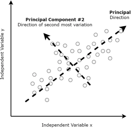
2.1 Principle component analysis

[image:26.595.157.375.476.690.2]

Principle component analysis is a dimensional reduction technique that project high dimensional data to different directions into vectors. The total number of data dimensions is the total number of principle components where the first principle component representing the most variance of the data set and the second principle component representing the second largest variance etc. A simple figure example can be found in Figure 2.1. This technique is used in this project to select the variables that represent the most variance of the whole variables. This is done by calculating the correlation between the variables and the first principle components. The higher the correlations are, the more important the variable is.

(27)

2.2 Artificial Neural Network

Artificial Neural Network is an interconnected system that can learn from samples. It is inspired by biological neural network. An example graph is shown in Figure 2.2. Each neural network consists of an input layer, output layer, hidden layer and biased nodes. Each node has its activation function and on each neuron there is an assigned weight. In our case, the initial weights are chosen at random. The weights are updated each time it get through a node with activation function. The activation function we use here is the following logistic function:

Sigmoid(z) = 1

1 +e−z (2.1)

Sigmoid function is widely used because it always return a value that is between 0 and 1 thus it is a good representative of probability used for binary step function. A binary step function means that if the value is above a certain value known as the threshold, the output is activated, otherwise it is not activated. The final prediction value is the sum of the weights multiplied by the corresponding input

Figure 2.2: Artificial Neural Network

plus bias value formulated as follows:

P rediction=X(weight∗input) +bias (2.2)

(28)

2.3 Random Forest

Random forest is an extension of decision tree. The model aggregates the prediction made by multiple decision trees of varying depth. Each tree is trained on a subset of the data set. The portion of samples that were left out all named Out-Of-Bag data set which is used for the model to evaluate itself. Random forest in R deciding on the criteria to split a tree by measuring the impurity produced by each feature. The impurity is indicated by Gini index or entropy. The prediction result is produced by taking the average of the predictions made by each decision tree in the forest.

Figure 2.3: Random Forest

2.4 Partial Least Squared Regression

Partial Least Squared Regression (PLSR) is a statistical method that finds a linear regression model by projecting the independent variables and dependent variables to a new space. It belongs to the Partial Least Squared (PLS) models family. According to (Heberger, 2008), PLS model is a bi-linear method where information in the original data set X is projected into a small number of latent vari-ables to ensure that the first components are those that are most relevant for predicting Y varivari-ables. This make it close to the idea of principle component analysis and principle component regression. The mathematics formulation of PLS model is the following:

X=T ∗PT +E (2.3)

Y =U ∗QT +F (2.4)

(29)

CHAPTER

THREE

DATA COLLECTION

In this chapter we will introduce the data source and parameters that is currently exist and potentially usable for this project. Data are primarily cleaned and integrated for first glance. Investigation on the meaning of the data has been conducted. In addition, part of the relation among parameters has been checked to verify the quality of the data source. A full data dictionary can be found in appendix A. Four separated data logger systems are currently logging data for the Galv line namely are Set up sheet(section 2.1), Data warehouse(section 2.2), IBA(section 2.3) and EMASS(section 2.4). Data integration tool is introduced in section 2.5.

3.1 Set up sheet

Setup sheet is the only data source where data are manually measured and logged. It is used for engineers to track parameters of maintenance cycles. The data are component related data such as roll diameter, whether the bush is new when installed and whether the sleeves are coated. The bush wear has been recorded after each campaign (approximately every 4 weeks). By the end of the data collection phase 6 samples of bush wear measurement is available from 15/05/2019 to 12/09/2019. By the end of the project 3 additional samples becomes available that are used for validation purpose. 15 variables are logged including date and time. The data logged on set up sheet are not continuous and need to be further processed into continuous data points before implementing. Furthermore, as the data are logged manually, human errors are not avoidable especially the bush wear measurement that is being used as target variable.

3.2 Data warehouse

Data warehouse is logging procurement and product property related data. Two interface within data warehouse called ”SIMPPS” and ”NEMO” has been investigated as these two interface has been suggested the most relevant by domain expert. Data from 15-05-2019 to 12-09-2019 has been extracted corresponding to the maintenance cycles. Respectively 95 variables and 110 variables are ex-tracted and they are with different number of observations, 4232 observations in ”SIMPPS” and 20232 observations in ”NEMO”. As there are some parameters with no data logged at all, or only few ob-servations are logged, we have excluded them and only leave the parameters with continuously logged value. In total 93 variables are left for further investigation. After investigated the meanings of these variables, we select the variables that eventually used for modeling based on literature survey findings.

(30)

Time spots from different interface are logged differently only very few data are logged at the same time. Some parameters share the same meaning but with different names such as coil width. There are in total 4 parameters that indicate coil width. They are however can’t be interpreted logically as the most of the finished coil width are logged larger than the ordered and received coil width from supplier. This according to firm expert is not logical as the coil are stretched during the process thus the width should be narrower. Conclusion can be drawn that if it is not the coil width that is logged wrong, it is then the coil ID was messed up. As this flaw is happening in a large margin and the fact that the widths data are all sharing the same trend the possibility that the coil IDs are logged wrong is low. This further reflects the data quality of data warehouse has a large space for improvement. In the end coil length, scrape length and surface area related variables are collected and used for prediction purpose. The reasoning for this is explained in Chapter 6

3.3 IBA

Data from IBA are system related corresponds to the the air-knives and the bath. The data are coming from sensors that has been installed within the system. We have extracted all the parameters available from the IBA starting from January 2019 to September 2019. The data file is over 10 GB in text file format.

As a first glance, we discovered that from 01-01-2019 to 17-03-2019, the data weren’t logged correctly, as the data are either logged as ”1” or ”nan”(not a number). From 17-03-2019, the data are all logged in numerical format. 12 data points are logged per minute and that is the main reason why the data file is huge. Moreover, 694 variables are logged representing various blocks in the control loop. According to the domain expert, only variables that marked as input are relevant for the air-knife behaviors. Base on that, 81 variables are left for further investigations. 3,119,156 observations are logged from March to September 2019. As a preliminary judgement, there are few missing data points each parameter and few parameters with the same data but different labels. These quality issues will not effect the analysis as they can be easily cleaned.

3.4 EMASS

EMASS system is a brand new system that has just been implemented from January 2019 to stabilise the strip. The system logged features from the strip such as strip width, length and vibrations. The system current are also logged which indicates how hard the system works. 16 sensors exist on EMass with 8 sensors on each side of the strip logging distances of the strip to the sensor. Currents in the sensors are also logged. Data files per day are logged into 7Z file format. Thus these data files has to be compressed into a folder before opening. After open the folder, there are approximately 200 text files were logged per day. There are in total 5 million to 6 billion observations per day and the total data size in EMASS is 43GB. Thousands of data points are logged per minute with inconsistent logging intervals. More over, the operators shut down the system every 12 hours to clean the machine. Depending on the shut down time span, it make sense that the total number of observations per day differs.

3.5 Data cleaning and integration

(31)

sets, however, the memory space is not large enough to handle data from EMASS, not even half day data. For the same reason other data cleaning tool wasn’t good enough for our case either.

In the end data are integrated from different data source using statistical software R. Specific variables from Set up sheet, Data Warehouse and IBA are selected for predictive model building. Detailed data reading, selection and integration process can be found in Chapter 5 and Chapter 6.

3.6 Conclusion

To conclude the report so far, the first research questions (question 1a-1d) is answered as follows:

1a.What is the current maintenance process in Tata Steel Shotton?

In general maintenance decisions have been made based on experience in Tata Steel Shotton. Specifi-cally, the current maintenance cycle of the pot gear, current maintenance cycle is approximately four weeks when there are no other faults such as strip break occurs. At the end of every four weeks, the line will be shut down and the pot gear will be replaced even if there hasn’t been any failure. Engineers has been trying out larger bush diameters to prolong the maintenance cycle.

1b-c.What are the existing data that ready for collection and what what are the meaning of the existing data?

In total four separate systems are in use to collect data from different perspective. The four data sources are: Set up sheet, Data warehouse, IBA and EMASS. Set up sheet records data regarding component properties such as roll diameter, roll condition before in line and bush condition. Bush wear data are logged after each maintenance cycle from 15-05-2019. The data in set up sheet are logged manually thus human measurement errors are hard to avoid and should be considered when further analyzing

Data warehouse records mainly procurement related data, such as the product the customer ordered, the product delivered, the team ID and batch ID etc. The data from different interface in data ware-house are not logged at the same time point. Some parameters such as ”coil width” appear repetitively but can’t be interpreted logically, for example, the finished coil width is supposed to be narrower than ordered and received coil width but they are logged larger. Such phenomenon to certain extent reflects the poor data quality in data warehouse.

1d.How can the data from different sources be integrated?

Statistical software ”R” has been used for data reading, cleaning and integration. Because R is capable of handling the data size from EMASS system while the rest of the tools such as OpenRefine has been tried out but failed to do so.

(32)

STATE OF ART

Over fifty papers has been reviewed in this chapter to present a view on the current research status in predictive maintenance in terms of component wear. Section 3.1 explores the general position of predictive maintenance in industry 4.0 concept. Section 3.2 explores physics behaviour of metal to metal contact wear to extract insight on the cause of wearing. Section 3.3 presents a broad review of data driven methods that have been used to predict component wear. Section 3.4 is focused on techniques for independent variables selections and feature extraction. The required data structure for modeling has also been reviewed. Current research gaps in predictive maintenance in component wear has been presented in section 3.5.

4.1 Predictive maintenance in industry 4.0

(33)

explanatory power and suitable when data set has high dimensions,however, it is prone to overfit. ANN, DNN and AE have achieved more than 97% accuracy in 80% literature. It also concludes that when using deep learning(DL) algorithms, deeper network architecture and higher dimensional feature vectors are more significant in improving the performance.

4.2 Mechanical contact wearing behaviour

As the goal of this project is mainly investigating the predictive maintenance on wearing condition, literature surveys have been done to explore the cause of mechanical degradation, especially metal to metal contact wear. In (Cubillo, 2016), metal-metal contact wearing behaviour is classified into two stages: adhesive wear and fatigue wear. Adhesive wear is due to surface contact that leads to material transfer or loss from surface(Bayer, 2004). Fatigue wear however, generates surfaces cracks that after a critical number of cycles resulting in a severe damage. Adhesive wear can be modeled with the Archard’s law :

V olume[wear] =K∗ Load∗Slidingdistance

3∗M aterialhardness (4.1)

Where K is wear coefficient that can be adjusted to fit more complex wear models. Fatigue wear however can be modeled in different ways based on friction coefficient and lubrication factor. The main cause of fatigue wear is the force taken per unit area. Modeling formula for bearing wear with lubricating factor can be found in (Ocak, 2007). Bearing degradation behaviour has been investigated in (Wang, 2017) where the behaviour has also been classified into two stages, the first stage has been simulated with a normal random variableα with meanµand varianceα2 the second stage of degra-dation has been simulated with Geometric Brownian motion. Analysis of variance(ANOVA) was used to determine the effects of the machine parameters of surface roughness and flank wear. Linear and quadratic regression were applied to predict the outcome of the experiment. (Kivak, 2014). Similarly, (Hwang, 2015) did experiments and numerical study of wear in cross roller thrust bearings. In which the first stage of wear was concluded as linear wear with the Archard’s law. Failure such as spalling was concluded as non-linear wear. (Wang, 2014) applied enhanced particle filter to predict tool wear and the relationship between tool wear rate and the changes of applied load has been investigated which is only a modified differentiation equation of the the Archard’s law. In addition, tooling force was found to be increased as the tool gets worn. Normal load is proportional to the wear width, thus normal load can be approximated as linear relationship of wear width.

Summarising the findings, mechanical contact wear, material hardness, load, sliding distance and lubrication factor cause wearing and determine wear volumes(B K N Rao et al, 2012). The wearing behaviour mostly are classified into two stages, the first stage is linear wear whereas the second stage is nonlinear. It is found that load changes are proportional to the wear, indicating that the wear width forms a linear relation with the force at the stage. The second stage is more complex and usually leads to failure.

4.3 Data driven methods for wearing prediction

Methods for predictive maintenance in terms of wearing condition can be generally classified into three categories (Tobon-Mejia, 2012), namely mathematical model based method, experience based method and data-driven method. Mathematical modeling based method produces good results, but requires deep knowledge on system functions, which is a viewed as a disadvantage as it is often

(34)

hard to obtain. Experienced based method makes decisions based on empirical events and often pro-duces poor prediction results. Data driven based methods investigate the problem mainly from data perspective. Machine learning is often used to learn data patterns. Predictive maintenance using data driven method requires failure data as target variables and featured variables to describe input data(Gouriveau et al, 2013), however, failure data is often not available in industries as down times are prevented with the best efforts due to high down time cost.

Artificial neural network, support vector machine and random forest are the most implemented data driven methods. Besides, hidden Markov model(HMM) with strict data structures and reliable com-puting performance has also attracted lots of attentions. In recent years, many researchers have applied HMM in tool condition monitoring and achieved good results.(Liao, 2016) however, the data used for wearing prediction are mostly experimental data, which means machines are set up and run to failure for a number of times and data are collected by the sensors that installed on the machine. Thus critical parameters are fully obtained. Such ideal data sets are hard to get from real life.

Limited amount of study has concentrated on predictive maintenance with missing labels. (Zschech, 2019) investigated in prognostic model development with missing labels. It first uses unsupervised learning such as clustering techniques to create labels then use supervised learning namely Recur-rent neural network(RNN) to predict future labels. In (Amruthnath, 2018) unsupervised learning has been investigated to detect early fault in predictive maintenance on experimental data. T statistics, k-means clustering, c-means clustering and hierarchical clustering are implemented and compared. The result confirms that unsupervised learning can detect faulty behaviour and clustering results are similar. (R.Langone, 2015) proposed a least square support vector machine(Ls-SVM) framework for maintenance strategy optimization based on real-time condition monitoring. It used both clustering (unsupervised learning) and a supervised leaning method namely nonlinear auto-regression(NAR), however, with different data set, and conclude that supervised learning can achieve better result and meanwhile it is more computational expensive. Two methods combined may result in the optimised maintenance cost configuration.

Deep learning is also starting to be implemented for wearing prediction. In (Martinez-Arellano, 2019), convolutional neural network(CNN) in combination of time series imaging are implemented to predict wearing that can effectively detect the wearing condition and location.

Other studies such as (Zhao, 2017) and (Zhong, 2016) proposed using correlation analysis among dif-ferent sensor signals to detect early anomaly as they discovered that the distribution of sensors signals is likely to change when there is a faulty behaviour. Thus the correlation between sensors will change before anomaly truly happens. This way faulty behaviours can be detected in time for maintenance activities.

Evaluations of modeling performance are mostly based on prediction power. Classification models are evaluated with True positive(TF), False positive(FP) rate and accuracy(Li, 2004)&(Li, 2003)&(Susto, 2014). Regression models are often evaluated with mean squared error(MSE), residual and R squared value,(Wu, 2017). Some of the studies also put training time as one of the evaluation criteria.(Wu, 2017 and 2016). R square is calculated with the following formula:

R2 = 1−SumOf SquaresOf Residuals

T otalSumof Squares (4.2)

(35)

4.4 Data pre-possessing

A critical overview of wearing prediction using artificial neural network has been presented in (B K N Rao et al, 2012) where articles from 1997 to 2011 has been reviewed. Different data prepossessing techniques that described in the article are dimensional reduction techniques, data fusion methods, sta-tistical analysis and optimization algorithm for feature selection. Principle component analysis(PCA), multivariate methods etc are in the category of statistical analysis. PCA is the most implemented dimensional reduction technique.

Feature extraction and selection has been an active research area for deployment of artificial intel-ligence. In terms of prognostics, a dataset is expected to have a minimum sample size around 10 in order to perform data-driven modeling effectively.(Eker, 2012) Preferably, dataset for predictive maintenance should be able to describe several instances of the same fault in various different but similar components (Klein, University of Trier). In (Veltan, 2000) 72 wear volumes are generated in the datasets with experimental settings. PCA was used to reduce its dimension. In (Bolon-Canedo, 2011) two main approaches for feature extraction are presented as individual evaluation and subset evaluation. However it was claimed in the article that there is no best method. Efforts are focused on finding a good method for a specific problem area.

In (Javed, 2012) 315 wear measurements were produced with 16 features extracted from each mea-surement. In (Wang, 2015) 300 files were produced with each file corresponding to one cut. Force and vibrations in three directions are stored in the files. Pearson correlation coefficient is selected as a feature since, according to the author, a good feature should present consistent trend with wear propagation. Fisher’s discriminant ratio is also a feature selection technique that was implemented in (Xie, 2019) to extract features from cutting force. Statistical feature was used and wearing conditions were given labels: ’initial wear’, ’median wear’ and ’severe wear’. Some studies even skipped feature extraction step such as (Zhao, 2017), raw sensory signals are directly put into a CNN for wearing prediction. However, normalization is commonly used for data reprocessing (Kolodziejczyk, 2010) to first put data into a same scale. Genetic programming is used as an optimization algorithm to choose the best features and/or describe wear volume (Kolodziejczyk, 2010). Statistical features are widely used in wear prediction.(Zschech, 2019) extract time domain features: peak value, root mean square, standard deviation, kurtosis value, cxest factor, clearance factor, impulse factor and shape factor.

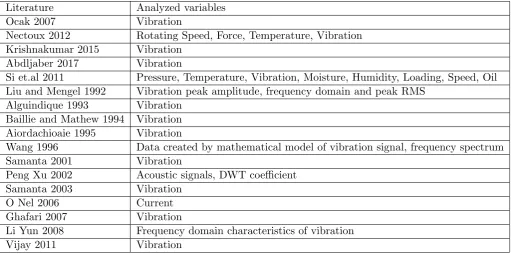
A table summarizing essential variales used for wearing predictions can be found in Table 4.1. Major-ity of wearing predictions are based on vibration analysis that is distinguished between time domain and frequency domain. Time domain vibration analysis extract time series features such as peak, rms, kurtosis and clearance value whereas frequency domain deploys spectrum analysis, envelope analysis and high frequency resonance technique(Eker, 2012).

Vibration signals are used as indicator of the condition. Vibration of 0.012 is considered as a refer-ence value to decide the change of tool.(Krishnakumar, 2015) Real time vibration based on structural damage was detected using one dimensional CNN in (Abdeljaber, 2017). The damage was detected and the location of the damaged joint was able to be detected. In (Y Shan, 2000) different prediction methods were applied to different bearing running stages to predict remaining life. Variables char-acterizing the state of deterioration are extracted for neural computation. Time domain vibration signals of rotating machinery with normal and defective bearings are used for wearing prediction in (Samania, 2001). Acoustic signals are used in(Xu 2002) and optimal statistical features are selected using a genetic algorithm. Current signature analysis are used in (O..Nel, 2006).

(36)

[image:36.595.57.569.116.370.2]

Table 4.1: Survey of essential variables

Literature Analyzed variables

Ocak 2007 Vibration

Nectoux 2012 Rotating Speed, Force, Temperature, Vibration Krishnakumar 2015 Vibration

Abdljaber 2017 Vibration

Si et.al 2011 Pressure, Temperature, Vibration, Moisture, Humidity, Loading, Speed, Oil Liu and Mengel 1992 Vibration peak amplitude, frequency domain and peak RMS

Alguindique 1993 Vibration Baillie and Mathew 1994 Vibration Aiordachioaie 1995 Vibration

Wang 1996 Data created by mathematical model of vibration signal, frequency spectrum

Samanta 2001 Vibration

Peng Xu 2002 Acoustic signals, DWT coefficient

Samanta 2003 Vibration

O Nel 2006 Current

Ghafari 2007 Vibration

Li Yun 2008 Frequency domain characteristics of vibration

Vijay 2011 Vibration

4.5 Gaps

Data cleaning and huge data set handling, according to (Bulletin 2000), should include: data anal-ysis, definition of transformation workflow and mapping rules, schema-related data transformation, verification, transformation and back-flow of cleaned data. These steps are provided as data cleaning guide to detect errors and inconsistency, transforming data into standard format with least possible manual inspections and verify the correctness of data transformation. Ideally, the cleaned data should replace the data in the original source. The approaches for data cleaning have never been presented in literature regarding predictive maintenance. Some results in articles are based on huge sensor-based data sets, for example, data sets with size 4TB(Li 2013). But how these data sets are read and cleaned are not presented. However, there are some techniques to clean sensor data such as weighted moving average(Zhuang, 2007) but it is implemented especially on small samples. In real life, sensor-based data sets are often huge and difficult to read. Thus it should require a long time to implement these techniques. In this report we present some techniques used to read large data sets in a reasonable amount of time and discuss how to reduce the file size and integrate data in chapter 5

Comparison of prediction result using different variables and reasoning of using vibration data in comparison with others are missing in literature. Almost all the papers were using vibration data to predict wearing condition without reasoning. Although using vibration data did produce good prediction results it is worth investigating that when vibration data is not available, are there other alternative parameters that could potentially replace vibrations and be used to predict wearing con-dition? Few papers analyzed on force and some combined several parameters(Kolodziejczyk, 2010) but no comparison study in terms of the prediction power with different parameters were conducted. Thus in this report we will also do some comparison in terms of predictive maintenance using different parameters and explore differences among results.

(37)

wear-Data driven solution to predictive maintenance

ing measurement. As mentioned before, most of the studies were conducted in labs, used data are experimental data. Most of the studies used multiple milling machines and let them run to failure and meanwhile the sensors installed on the milling machines are able to measure the wearing on the milling point, log vibrations and log forces from different dimensions. However, this ideal situation almost never happens in real industry setting. Take the cased used in this study as an example, there are no sensors can be installed around the bush as it is in a zinc pot. Thus vibrations and force both are not available, not to mention that the wearing measures are only able to be measured after every campaign. Some literature combines unsupervised and supervised technique to simulate target, but the result is hard to validate as there are only simulated labels exist. This study investigates the following: to what extent can predictive maintenance on wearing conditions be done with only partly available wearing measures and what other feasible predictive maintenance activities can be done with current available data.

4.6 Conclusion

By this end research question 2 is able to be answered to conclude predictive maintenance using data driven methods.

2a. Which data driven models have been used to predict metal contact wear in industries?

Data driven methods are mostly machine learning models. The most implemented machine learning models are random forest, support vector machine and artificial neural network. They all produce good prediction results on predicting failure(classification) or remaining use of life(regression). Arti-ficial neural network are the most implemented and is often modified into different structures. Other statistical based models can be considered as the overlap of empirical and data driven methods such as detecting correlation changes and distributions from historical data.

2b. What are the steps that has been used in literature in terms of data prepossessing and model building?

Classical method for predictive analytics is data collection, data cleaning, feature extraction and model building. Data sample required for model building in predictive analytics are samples covering variety of cases, with many predictive variables corresponding to one target variable.

Limited amount of studies concentrate on missing target issue as limited amount of studies are based on real life industrial data. Some studies compare different clustering techniques that are unsuper-vised machine learning models such that no target variables are required. However it is also falls out of predictive analytic category as unsupervised machine learning has descriptive nature. Some stud-ies combine unsupervised learning and supervised learning, specifically using clustering techniques to detect abnormal behaviour and making different labels for training set and then training predictive models using training set with simulated labels. The limitation of this method is that it is hard to evaluate the predictive power as it can only be evaluated with simulated labels.

Feature extraction is an active research area as features extracted are likely to influence prediction result. Statistical features are the most widely used. Many algorithms are suitable to select optimal features such as principle component analysis and genetic algorithm. It has been concluded that no best technique exist for feature extraction it all depends on specific situations.

2c. What are the measures to evaluate predictive power of the models?

(38)

Predictive maintenance using data driven methods can be categorized into two categories as follows: -Classification: Predict system/component failure, the labels then can be set as: fail or not fail. Prediction power evaluation for classification models are True Positive rate, False Positive Rate and Accuracy measure.

-Regression: Predict system/component remaining use of life, wearing millimeters etc. Prediction is a continuous variable. Prediction power is evaluated using MSE(mean squared error) and R squared value.

Some studies also take training time as one model selection criteria.

2d. Based on prediction power and current context which models are the most suitable for predictive maintenance?

When data availability is not a problem, random forest, support vector machine and neural network all show good prediction power. Random forest and support vector machine have their advantages that they are computational less expensive. Whereas neural network is more complex but then it is more flexible to suit different systems and conditions. It can even be used as an automatic feature extraction model and also powerful in deep learning for more detailed prediction such as recognizing the specific wearing location.

2e. What are the gaps and limitations of current literature on predictive maintenance in industry? Current studies on predictive maintenance barely describe the size of data set and how to read huge data set. Most of the data cleaning techniques are tested on small data samples which is far from real life situation. As in real life, sensor data are logging at a high frequency and the data file are huge and not even be able to read by software. Not to mention implementing techniques to clean them.

Most of the predictive maintenance on wearing conditions only use one parameter namely vibration signals as it is always produce good prediction result. Few studies uses other parameters based on physical property of the component. However, sometimes none of these parameters are available, thus alternative parameters to predict bush wear are worth investigating.