Performance analysis of spectrum sensing with multiple primary users

University of Warwick institutional repository: http://go.warwick.ac.uk/wrap

This paper is made available online in accordance with publisher policies. Please scroll down to view the document itself. Please refer to the repository record for this item and our policy information available from the repository home page for further information.

To see the final version of this paper please visit the publisher’s website. Access to the published version may require a subscription.

Author(s): Bo Zhao, Yunfei Chen, Chen He and Lingge Jiang

Article Title: Performance Analysis of Spectrum Sensing With Multiple Primary Users

Year of publication: 2012 Link to published article:

http://dx.doi.org/10.1109/TVT.2012.2183010

Publisher statement: “© 2012 IEEE. Personal use of this material is permitted. Permission from IEEE must be obtained for all other uses, in any current or future media, including reprinting/republishing this

material for advertising or promotional purposes, creating new

Performance Analysis of Spectrum Sensing

With Multiple Primary Users

Bo Zhao, Yunfei Chen, Senior Member, IEEE, Chen He, Member, IEEE, Lingge Jiang,

Member, IEEE

Corresponding Address:

Yunfei Chen

School of Engineering

University of Warwick, Coventry, U.K. CV4 7AL

Tel: +44 (0)24 765 23105,

e-mail:

[email protected]

Abstract

The effect of multiple primary users on the spectrum sensing performance is investigated. Different

models for the primary user traffic are considered. The effects of different system parameters on

the sening accuracy are examined. Numerical results show that the spectrum sensing performance is

significantly degraded by the primary user traffic, and that the degradation decreases when the number

of primary users increases.

Index Terms

Cognitive radio, primary user traffic, spectrum sensing.

Bo Zhao and Yunfei Chen are with the School of Engineering, University of Warwick, Coventry, U.K. CV4 7AL (e-mail:

{Bo.Zhao, Yunfei.Chen}@warwick.ac.uk)

Chen He and Lingge Jiang are with the Department of Electronic Engineering, Shanghai Jiao Tong University, Shanghai,

I. INTRODUCTION

Spectrum sensing is a critical functionality of cognitive radio [1]. It enables unlicensed users,

referred to as cognitive radio (CR) users hereafter, to find the “spectrum holes”. Many works have

been conducted on spectrum sensing [2] - [4]. Among them, energy detector is the most widely

used method. All these previous works assume that the primary user is either absent or present

during the whole sensing period. However, in practice, the primary user may arrive or leave

during the sensing period. The effect of the primary user traffic on the sensing performance has

been analyzed in [5] for the case when only one primary user occupies the licensed spectrum at a

time. In [6], the energy detection was improved to reduce the effect from the primary user traffic

when only one primary user is present. However, in many widely used code division multiple

access (CDMA) systems, such as 3G and WiMAX, the systems are designed to have several users

operating in the same frequency band simultaneously. The “spectrum holes” also include vacant

unlicensed bands. In this case, several unlicensed systems, such as Wi-Fi, Bluetooth and DECT,

will share the same band without coordination, giving the scenario where multiple primary users

may occupy the same band. All these realistic applications motivate a general investigation of

the effect of primary user traffic on the sensing performance with multiple primary users.

In this letter, the effect of primary user traffic on the performance of energy detection is

evaluated by considering the general case when multiple primary users arrive or leave during the

sensing period. Different models for the primary user traffic are considered. Numerical results

show that the performance of energy detection is significantly degraded when the primary user

status changes during the sensing period, and that the degradation decreases when the number

of primary users increases.

II. SYSTEMMODEL

In the energy detection, the output of a band-pass filter with bandwidth W is squared and

is _Y = P2m

n=1Yn2, where Yn = Zn when the n-th sample does not contain the primary signal

and Yn =S( u)

n +Zn when the n-th sample does contain the primary signal, Zn are independent

samples of the additive white Gaussian noise (AWGN) with mean zero and variance α2_{, and}

Sn(u) are samples of the signals from uprimary users. It is assumed that each primary user signal

is independent and identically distributed with average power P. Thus, the average SNRs for one primary user and u primary users areγ =P/α2 _{and uγ, respectively. In the case when the}

primary user signal is non-identically distributed, γ and uγ can be replaced by γi for the i-th

primary signal and Pu

i=1γi in the following results, respectively.

Each primary user has two status: busy or idle. The holding time of busy or idle is assumed

to be random and has cumulative distribution functions (CDFs) Fλ(x) or Fµ(x), respectively.

Denote the mean holding times of busy and idle as λ and µ, respectively. Therefore, at any

time instant, a primary user is busy with probability pb(λ, µ) = _µ+λ_λ, and idle with probability

pi(λ, µ) = 1−pb(λ, µ). Assume that a primary user is idle at the beginning of the sensing period,

and then becomes busy after the k-th sample. Then, the last sample of the idle period is the k-th sample. The probability mass function (PMF) for the case when the primary user’s status

changes from idle to busy after the k-th sample is derived as [9]

pµ(k) = Fµ(kTs)−Fµ((k−1)Ts) (1)

where Ts is the sample interval. Similarly, the PMF for the case when the primary user’s status

changes from busy to idle after the k-th sample is derived as

pλ(k) = Fλ(kTs)−Fλ((k−1)Ts). (2)

Note that this alternating renewal process model has been verified by real traffic data [7] [8] and

has been used in different works [9]- [11]. Therefore, our analysis based on this model applies

to these practical cases [7]- [11]. As well, since the analysis is based on a very general traffic

model in (1) and (2), it is valid for any model of the primary network with a specific PMF.

In the numerical examples, several typical models will be examined but study of each primary

III. PERFORMANCE ANALYSIS

Assume that the state of each primary user changes at most once during the sensing period.

This is the case when the sensing period is at the same level of the holding time but also the

case when the sensing period is shorter than the holding time but the primary user happens to

change status during the sensing period. We consider the case of two primary users first. In this

case, at any time instant, the channel can be idle with probability pI(λ, µ) = p2i(λ, µ), or be

occupied by one primary user with probability pB1(λ, µ) = 2pi(λ, µ)pb(λ, µ), or be occupied

by two primary users with probability pB2(λ, µ) = p2b(λ, µ). Since the state of each primary

user changes at most once during the sensing period, the channel state can change up to twice

during the sensing period. Then, the binary hypothesis testing problem in the conventional energy

detector given by [2] can be decomposed into a ten-hypothesis testing problem as

Y =                                                                 

P2m

n=1(S (2)

n +Zn)2, H1,1

Pk1

n=1(S (1)

n +Zn)2+P2_nm_=k1+1(Sn(2)+Zn)2, H1,2

Pk1

n=1(S (2)

n +Zn)2+P2_nm_=k1+1(Sn(1)+Zn)2, H1,3

P2m

n=1(S (1)

n +Zn)2, H1,4

Pk1

n=1Zn2+

P2m

n=k1+1(S

(1)

n +Zn)2, H1,5

Pmin(k1,k2)

n=1 Zn2+

Pmax(k1,k2)

n=min(k1,k2)+1(S

(1)

n +Zn)2+P2_nm_{=max(k1,k2)+1}(Sn(2)+Zn)2, H1,6

Pmin(k1,k2)

n=1 (S (1)

n +Zn)2+P_nk2_=k1+1Zn2+

Pk1

n=k2+1(S

(2)

n +Zn)2

+P2m

n=max(k1,k2)+1(S

(1)

n +Zn)2, H1,7

P2m

n=1Zn2, H0,1

Pk1

n=1(S (1)

n +Zn)2+P2_nm_=k1+1Zn2, H0,2

Pmin(k1,k2)

n=1 (S (2)

n +Zn)2+P

max(k1,k2)

n=min(k1,k2)+1(S

(1)

n +Zn)2+P2_nm_{=max(k1,k2)+1}Zn2, H0,3

(3)

where k1 represents the number of samples after which the first primary user’s status changes,

k2 represents the number of samples after which the second primary user’s status changes, k1

and k2 are determined by the primary user traffic and k1, k2 ∈[1,2m], Sn(1) is the primary user

as before, and Pb

i=a(·) = 0 when a > b. One sees that the conventional sensing model in [2]

corresponds to the hypotheses of _H1,4 and H0,1 in (3), and the sensing model for one primary

user in [5] corresponds to the hypotheses of _H1,4, H1,5, H0,1 and H0,2 in (3).

The probabilities of detection and false alarm can be derived as

Pd(λ, µ) =

1

P(_H1){

P(_H1,1, λ, µ)·P(H1|H1,1) +P(H1,4, λ, µ)·P(H1|H1,4) (4)

+

2m

X

k1=1

[P(_H1,2, λ, µ, k1)·P(H1|H1,2, k1) +P(H1,3, λ, µ, k1)·P(H1|H1,3, k1)

+P(_H1,5, λ, µ, k1)·P(H1|H1,5, k1) + 2m

X

k2=1

(P(_H1,6, λ, µ, k1, k2)·P(H1|H1,6, k1, k2)

+P(_H1,7, λ, µ, k1, k2)·P(H1|H1,7, k1, k2))]}

and

Pf(λ, µ) =

1

P(_H0){

P(_H0,1, λ, µ)·P(H1|H0,1) + 2m

X

k1=1

[P(_H0,2, λ, µ, k1)·P(H1|H0,2, k1) (5)

+

2m

X

k2=1

P(_H0,3, λ, µ, k1, k2)·P(H1|H0,3, k1, k2)]},

respectively, where

P(_H1) =P(H1,1, λ, µ) +P(H1,4, λ, µ) + 2m

X

k1=1

[P(_H1,2, λ, µ, k1) +P(H1,3, λ, µ, k1) (6)

+P(_H1,5, λ, µ, k1) + 2m

X

k2=1

(P(_H1,6, λ, µ, k1, k2) +P(H1,7, λ, µ, k1, k2))]

is the probability that the channel is occupied, and

P(_H0) =P(H0,1, λ, µ) + 2m

X

k1=1

[P(_H0,2, λ, µ, k1) + 2m

X

k2=1

P(_H0,3, λ, µ, k1, k2)] (7)

is the probability that the channel is idle, P(_H1,1, λ, µ), P(H1,2, λ, µ, k1), P(H1,3, λ, µ, k1),

P(_H1,4, λ, µ),P(H1,5, λ, µ, k1),P(H1,6, λ, µ, k1, k2),P(H1,7, λ, µ, k1, k2),P(H0,1, λ, µ),P(H0,2,

λ, µ, k1) and P(H0,3, λ, µ, k1, k2) are defined in Appendix A. Note from (4)-(7) that the

applies to all applications. The specific value of P˜ could be low or high, depending on the specific sensing period and primary mean holding time in the interested applications.

The above analysis can be specialized to the primary networks with λ << µ by setting pB1(λ, µ) = 0 and pB2(λ, µ) = 0 in the equations, as pb(λ, µ)≈ 0 and pi(λ, µ) ≈ 1. It applies

to the case of two primary users. Using similar methods, one can extend it to the case of more

primary users. The complexity grows exponentially with the number of primary users. Thus, it

does not lead to a tractable analysis for a large number of primary users. On the other hand, a

simplified special case exists when λ equals µ. One can let k1 and k2 span from 0 to 2m and

define pµ(0) = 1−Fλ(T), pλ(0) = 1−Fµ(T). Then, one has the case of N primary users as

Y =                                                                 

Pk1

n=1Zn2+

Pk2

n=k1+1(S

(1)

n +Zn)2

+Pk3

n=k2+1(S

(2)

n +Zn)2+...+P2_nm_=kN+1(S

(N)

n +Zn)2, H1,1

..

. ...

Pk1

n=1(S (i−1)

n +Zn)2+P_nk2_=k1+1(S( i−2)

n +Zn)2+· · ·

+Pki −1

n=ki₋2+1(S

(i−(i−1))

n +Zn)2+Pk

i

n=ki₋1+1Z

2

n+

Pki+1

n=ki+1(S

(1)

n +Zn)2

+Pki+2

n=ki+1+1(S

(2)

n +Zn)2+· · ·+P2_nm_=kN+1(S

(N−(i−1))

n +Zn)2, H1,i

..

. ...

Pk1

n=1(S (N−1)

n +Zn)2 +P_nk2_=k1+1(S( N−2)

n +Zn)2+· · ·

+PkN

n=kN −1+1

Z2

n+

P2m

n=kN+1(S

(1)

n +Zn)2, H1,N

Pk1

n=1(S (N)

n +Zn)2+P_nk2_=k1+1(S( N−1)

n +Zn)2+· · ·

+PkN

n=kN −1+1

(S(N−(N−1))

n +Zn)2+P2_nm_=kN+1Z

2

n, H0

(8)

where _H1,i represent the hypothesis that the channel is occupied by N −(i−1) primary users

at the end of the sensing period, _H0 represent the hypothesis that the channel is idle at the end

of the sensing period, k1,· · ·ki,· · ·kN ∈ [0,2m] represents the number of samples after which

The probabilities of detection and false alarm in this case are derived in Appendix B as

Pd(λ, µ) =

1

P(_H1)

[

2m

X

k1=0

2m

X

k2=0 · · ·

2m

X

kN=0

P(_H1,1, λ, µ, k1,· · · , kN)·P(H1|H1,1, k1,· · · , kN) +· · ·

+P(_H1,N, λ, µ, k1,· · · , kN)·P(H1|H1,N, k1,· · · , kN)] (9)

and

Pf(λ, µ) =

1

P(_H0)

[

2m

X

k1=0

2m

X

k2=0 · · ·

2m

X

kN=0

P(_H0, λ, µ, k1,· · · , kN)·P(H1|H0, k1,· · · , kN)] (10)

respectively, where

P(_H1) = 2m

X

k1=0

2m

X

k2=0 · · ·

2m

X

kN=0

P(_H1,1, λ, µ, k1,· · · , kN) +· · ·+P(H1,N, λ, µ, k1,· · · , kN) (11)

is the probability that the channel is occupied,

P(_H0) = 2m

X

k1=0

2m

X

k2=0 · · ·

2m

X

kN=0

P(_H0, λ, µ, k1,· · · , kN) (12)

is the probability that the channel is idle, and the expressions of P(_H1,1, λ, µ, k1,· · · , kN), · · ·,

P(_H1,N, λ, µ, k1,· · · , kN)andP(H0, λ, µ, k1,· · · , kN)are given in Appendix B. Then, the error

probability can be calculated as

Pe(λ, µ) = [1−Pd(λ, µ)]P(H1) +Pf(λ, µ)P(H0). (13)

Note that the above results assume the same traffic load for all primary users. It can be easily

extended to the case when different primary users have different loads by replacing λ and µ

with λi and µi, respectively, for the i-th user.

IV. NUMERICAL RESULTS ANDDISCUSSION

In this section, numerical examples are presented. In the Neyman-Pearson (NP) criterion,η is

calculated by assigning a predetermined value β to the probability of false-alarm derived [12].

In the minimum error-probability (ME) criterion, η is calculated by minimizing the probability

of error [12]. We set Ts= 0.00125s in all the examples. Exponential distribution [13], Gamma

distribution [14] and lognormal distribution [15] are used to model the primary user traffic. Also,

used but it still gives very useful and important insights on the sensing performance, which

serves the purpose of this paper.

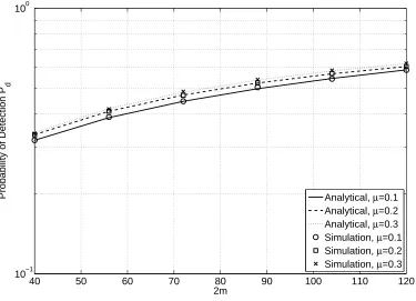
Fig. 1 compares the simulation results and the analytical results for the probability of detection Pd. Two primary users are considered with exponential traffic,γ =−5 dB, and the NP criterion

for β = 0.01. One sees that the simulation results agree with the analytical results well for all the cases. Comparing different values of µ, it can be seen that, the larger the value of µis, the

higher the probability of detection will be, under the same conditions. This is due to the fact

that, the larger the mean holding time is, the less the probability that the primary user status

changes during the sensing time will be, which improves the detection performance.

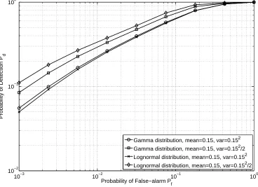
Fig. 2 shows the receiver operating characteristics (ROC) curves for different models of the

primary user traffic based on the NP criterion. In the calculation, the detection threshold η is

derived from (5) numerically, by varyingPf from10

−3

to 1. Also, we haveT = 0.05s andγ = 0 dB. Comparing the ROC curves for the same distribution with different variances, one sees that

a smaller variance gives a higher Pd for the same Pf. This is because when the mean holding

time is larger than the sensing time, a smaller variance makes the probability of a primary user

status changes during the sensing period smaller and therefore, the sensing performance is better.

Comparing the ROC curves for different distributions, it is seen that the sensing performance for

the lognormal distributed holding time is more sensitive to the variance than that for the Gamma

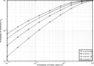
distributed holding time. For the same system, in Fig. 3, we take the exponential holding time as

an example to show the effect of the mean holding time on the spectrum sensing performance.

One can see that a smaller mean holding time results in a lower Pd for the same given Pf.

This is due to the fact that a smaller mean holding time makes it more likely for the primary

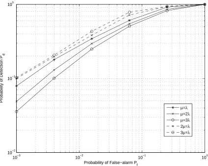
user status to change during the sensing period and to degrade the sensing performance. Fig. 4

shows the ROC curves for different relationships between µ and λ for two primary users when λ= 0.2. When λ is fixed to 0.2, it can be seen from the figure that a smaller value of µ gives a better ROC performance. However, the performance gain is smaller when µ is smaller.

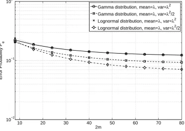
primary user traffic. Two primary users are considered. The mean holding time in this figure is

determined by the ratio R =λ/T, and we set R = 3 in this comparison. We have γ = 0 dB, and the ME criterion is used. It can be observed that a smaller variance results in a lower error

probability, and the error probability for the lognormal distributed holding time is more sensitive

to the variance than that for the Gamma distributed holding time. It can also be shown that a larger R results in a lower error probability. This is because that, the larger the value of R is,

the smaller the probability that a primary user status changes during the sensing period will be.

Also one can show that the error probability for a larger R is more sensitive to the number of

samples than that for a smaller R.

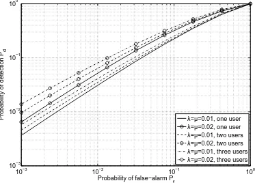
Fig. 6 shows the ROC curves for different numbers of primary users. The NP criterion is

used with Pf varying from 10

−3

to 1. We set T = 0.01 s, γ = 0 dB, and the holding time is exponentially distributed with means 0.01 s and 0.02 s. As expected, a larger number of primary users results in a higher probability of detection under the same conditions. Comparing

the performance gains achieved by multiple primary users for different values of mean holding

time, it is seen that a larger mean holding time increases the performance gain.

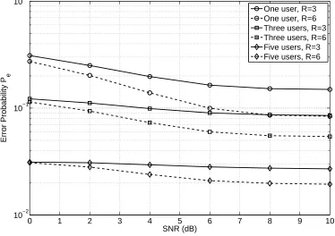
Fig. 7 shows the error probability versus the SNR of the primary signal for different numbers

of primary users. We setT = 0.01s, and the mean holding time in this figure is also determined by the ratio R=λ/T, which is set at 3 and 6 in this comparison. It is seen that the decreasing rate of the error probability for R = 3 is smaller than that for R = 6. This is also due to the fact that a smallerR results in a higher probability that the primary users arrive or leave during

the sensing period. Also, as expected, a larger number of primary users results in a lower error

probability under the same conditions.

V. CONCLUSIONS

The effect of the primary user traffic on the performance of spectrum sensing has been analyzed

for the case when multiple primary users arrive or leave during the sensing period. Numerical

user traffic and the degradation decreases when the number of primary users increases. This

analysis tells us how spectrum sensing will perform for a given traffic and a given number of

primary users. However, knowledge of the traffic distribution and the number of primary users

is not required in the energy detection. Although this paper extends the single-user case in [5]

using a common method, to the best of the authors’ knowledge, the result is new and has not been obtained in the literature. Due to the exponential complexity for an arbitrary number of

primary users, this paper only presents a simplified result for λ = µ. Although this result is useful and important, future research will derive general closed-form expressions for any values

of mean holding times by considering approximations to the hypotheses-testing problem.

APPENDIXA

DERIVATIONS OF (4)AND(5)

Based on the traffic model given in (1) and (2), and assuming that two primary users are

independent, the probability for each channel state can be calculated as

P(_H1,1, λ, µ) = pB2(1−Fλ(T))(1−Fλ(T)) (14)

P(_H1,2, λ, µ, k1) =pB1pµ(k1)(1−Fλ(T))

P(_H1,3, λ, µ, k1) = 2pB2(1−Fλ(T))pλ(k1)

P(_H1,4, λ, µ) =pB1(1−Fλ(T))(1−Fµ(T))

P(_H1,5, λ, µ, k1) = 2pI(1−Fµ(T))pµ(k1)

P(_H1,6, λ, µ, k1, k2) = pIpµ(k1)pµ(k2)

P(_H1,7, λ, µ, k1, k2) = pB1pµ(k1)pλ(k2)

P(_H0,1, λ, µ) =pI(1−Fµ(T))(1−Fµ(T))

P(_H0,2, λ, µ, k1) =pB1pλ(k1)(1−Fµ(T))

Similar to [5], chi-square distribution is used to model the output of the energy detector _Y.

Using this distribution, the probability of detection under different cases can be derived as

P(_H1|H1,1) = Qm(

p

4mγ,√η), P(_H1|H1,2, k1) = Qm(

p

(2m₋k1)γ+ 2mγ,√η) (15)

P(_H1|H1,3, k1) = Qm(

p

k1γ+ 2mγ,√η), P(H1|H1,4) =Qm(

p

2mγ,√η)

P(_H1|H1,5, k1) =Qm(

p

(2m₋k1)γ,√η)

P(_H1|H1,6, k1, k2) =Qm(

p

(2m₋k1)γ+ (2m−k2)γ,√η)

P(_H1|H1,7, k1, k2) =Qm(

p

k1γ+ (2m−k2)γ,√η)

where_Qm(a, b) =

R∞

b xm

am −1e

−x

2_+a2 2 I

m−1(ax)dxis the generalized Marcum Q-function [16] with

Im−1(·)being the modified Bessel function of the (m−1)th order, andηis the detection threshold

for the energy detector. The probability of false alarm under different cases are given as

P(_H1|H0,1) = 1−

Γ(m, η/2)

Γ(m) (16)

P(_H1|H0,2, k1) =Qm(

p

k1γ,√η)

P(_H1|H0,3, k1, k2) = Qm(

p

k1γ+k2γ,√η),

where Γ(z) =R∞

0 t

z−1

e−t

dt and Γ(z, x) = Rx

0 t

z−1

e−t

dt are the complete and lower incomplete

Gamma functions [17], respectively. Note that the probabilities of false alarm and detection given in (15) and (16), respectively, are conditional probabilities, conditioned on k1 and k2. By

averaging the conditional probabilities of detection in (15) and the conditional probabilities of

false alarm in (16) over k1 and k2, the overall unconditional probabilities of detection and false

alarm can be calculated as (4) and (5), respectively.

APPENDIX B

DERIVATIONS OF (9)AND(10)

Using the chi-square distribution for _Y in (8), by inspection, _Y in _H1,i has freedom 2m and

probability of detection for different cases in (8) can be calculated as

P(_H1|H1,i, k1, ..., kN) =

Qm(

p

(2m₋k1)γ+...(2m−kN−i+1)γ+kN−i+2γ+...+kNγ, √_η)

for i= 1,_{· · ·} , N. Similarly, the probability of false alarm can be calculated as

P(_H1|H0, k1,· · · , kN) = 1−

Γ(m, η/2)

Γ(m) , when k1 =k2 =· · ·=kN = 0 (17)

P(_H1|H0, k1,· · · , kN) = Qm(

p

k1γ+k2γ+· · ·+kNγ,√η) otherwise.

Next, we calculate the probabilities of the N + 1 channel states. When there are N primary users, at the beginning of the sensing, the channel has N + 1 possible states with probabilities

pBi = Ni

pib(λ, µ)p N−i

i (λ, µ) (18)

pI = NN

pNi (λ, µ)

where pBi is the probability that i primary users are busy and other primary users are idle,

i = 1,_{· · ·} , N, and pI is the probability that all the primary users are idle. Since each primary

user’s status changes at most once during the whole sensing period, the channel status changes

up to N times when there are N primary users. Then, one as

P(_H1,i, λ, µ, k1, ..., kN) =pB(i−1)

N−i+1

Y

n1=1

pµ(kn1)·

i−1

Y

n2=1

pλ(kn2)

P(_H0, λ, µ, k1, ..., kN) =pBN N

Y

n=1

pλ(kn),

where P(_H1,i, λ, µ, k1, ..., kN) is the probability that i−1 primary users are idle and the rest

N ₋(i₋1) primary users are busy at the end of the sensing period, P(_H0, λ, µ, k1, ..., kN) is

the probability of that all theN primary users are idle at the end of the sensing period. Finally,

using the above results, the overall unconditional probabilities of detection and false alarm can

REFERENCES

[1] Z. Quan, S. Cui, H. V. Poor and A. H. Sayed, “Collaborative wideband sensing for cognitive radios,”IEEE Signal Processing

Mag., vol. 25, no. 6, pp. 60-73, Nov. 2008.

[2] D. Cabric, S. M. Mishra, R. W. Brodersen, “Implementation issues in spectrum sensing for cognitive radios,” inProc. the

38th. Asilomar Conference on Signals, Systems and Computers, pp. 772-776, Pacific Grove, CA, USA, Nov. 2004.

[3] S. Shellhammer and R. Tandra, “Performance of the power detector with noise uncertainty,” IEEE 802.22-06/0134r0, Jul.

2006.

[4] Y. Chen and N. C. Beaulieu, “Performance of collaborative spectrum sensing for cognitive radio in the presence of Gaussian

channel estimation errors”,IEEE Trans. Commun., vol. 57, no. 7, pp. 1944-1947, Jul. 2009.

[5] T. Wang, Y. Chen, E. L. Hins and B. Zhao, “Analysis of effect of primary user traffic on spectrum sensing performance”,

Proc. of the Fourth International Conference on Communications and Networking in China (ChinaCom 2009), pp. 1-5, Aug.

2009.

[6] N. C. Beaulieu and Y. Chen, “Improved energy detectors for cognitive radios with randomly arriving or departing primary

users”,IEEE Signal Process. Lett., vol. 17, no. 10, pp. 867-870, Oct. 2010.

[7] K. Sriram and W. Whitt, “Characterizing superposition arrival processes in packet multiplexers for voice and data,”IEEE

J. Sel. Areas Commun., vol. SAC-4, no. 6, pp. 833-846, Sept. 1986.

[8] X. Yang and A. P. Petropulu, “The extended alternating fractal renewal process for modeling traffic in high-speed

communication networks,”IEEE Trans. Signal Process., vol. 49, no. 7, pp. 1349-1363, Jul. 2001.

[9] J. Ma, X. Zhou and G. Y. Li, “Probability-based periodic spectrum sensing during secondary communication”,IEEE Trans.

Commun., vol. 58, no. 4, pp. 1291-1301, Apr. 2010.

[10] M. Sharma and A. Sahoo, “Opportunistic channel access scheme for cognitive radio system based on residual white space

distribution,” inProc. of the IEEE International Symposium on Personal Indoor and Mobile Radio Communications (PIMRC

2010), pp. 1842-1847, Instanbul, 26-30 Sept. 2010.

[11] P. Wang and I. F. Akyildiz, “Effects of different mobility models on traffic patterns in wireless sensor networks,” inProc.

of the IEEE GLOBECOM2010, pp. 1-5, Miami, U.S.A., 6-10 Dec. 2010.

[12] R. D. Yates and D. J. Goodman,Probability and Stochastic Processes, John Wiley&Sons, Inc., 1997.

[13] R. A. Guerin, “Channel occupancy time distribution in a cellular radio system,” IEEE Trans. Veh. Technol., vol. VT-35,

no. 3, pp. 89-99, Aug. 1987.

[14] Y. Fang, I. Chlamtac and Y.-B. Lin, “Call performance for a PCS network”,IEEE J. Sel. Areas Commun., vol. 15, no. 8,

pp. 1568-1581, Oct. 1997.

[15] C. Jedrzycki and V. C. M. Leung, “Probability distributions of channel holding time in cellular telephony systems”, in

IEEE Vehicular Technology Conference (VTC 96), pp. 247-251, Atlanta, GA, May 1996.

[16] A. H. Nuttall, “Some integrals involving the QM function,”IEEE Trans. Inform. Theory, vol. 21, no. 1, pp. 95-96, Jan.

1975.

40 50 60 70 80 90 100 110 120 10−1

100

2m

Probability of Detection P

d

Analytical, µ=0.1 Analytical, µ=0.2 Analytical, µ=0.3 Simulation, µ=0.1 Simulation, µ=0.2 Simulation, µ=0.3

Fig. 1. Probability of detectionPd versus the number of samples 2m based on the NP criterion.

10−3 10−2 10−1 100 10−2

10−1 100

Probability of False−alarm P

f

Probability of Detection P

d

Gamma distribution, mean=0.15, var=0.152 Gamma distribution, mean=0.15, var=0.152/2 Lognormal distribution, mean=0.15, var=0.152 Lognormal distribution, mean=0.15, var=0.152/2

10−3 10−2 10−1 100 10−2

10−1 100

Probability of False−alarm P

f

Probability of Detection P

d

λ=µ=0.05

λ=µ=0.1

λ=µ=0.15

λ=µ=0.2

Fig. 3. The ROC curves for different values of mean holding time of the primary user when the holding time is exponentially distributed based on the NP criterion. Two primary users are

10−3 10−2 10−1 100

10−2

10−1

100

Probability of False−alarm P f

Probability of Detection P

d

µ=λ µ=2λ µ=3λ 2µ=λ 3µ=λ

10 20 30 40 50 60 70 80 10−2

10−1 100

2m

Error Probability P

e

Gamma distribution, mean=λ, var=λ2 Gamma distribution, mean=λ, var=λ2/2

Lognormal distribution, mean=λ, var=λ2 Lognormal distribution, mean=λ, var=λ2/2

10−3 10−2 10−1 100 10−3

10−2 10−1 100

Probability of false−alarm P

f

Probability of detection P

d

λ=µ=0.01, one user

λ=µ=0.02, one user

λ=µ=0.01, two users

λ=µ=0.02, two users

λ=µ=0.01, three users

λ=µ=0.02, three users

Fig. 6. The ROC curves for different numbers of primary users and different values of mean holding time of the primary user when the holding time is exponentially distributed based on

0 1 2 3 4 5 6 7 8 9 10 10−2

10−1 100

SNR (dB)

Error Probability P

e

One user, R=3 One user, R=6 Three users, R=3 Three users, R=6 Five users, R=3 Five users, R=6