University of Warwick institutional repository:
http://go.warwick.ac.uk/wrap
A Thesis Submitted for the Degree of PhD at the University of Warwick
http://go.warwick.ac.uk/wrap/62032
This thesis is made available online and is protected by original copyright.
Please scroll down to view the document itself.
AUTHOR:Nicolai Peremezhney DEGREE: Ph.D.
TITLE: Chemical product/process design and optimization: development of novel techniques and integration of bio-feedstocks.
DATE OF DEPOSIT: . . . .
I agree that this thesis shall be available in accordance with the regulations governing the University of Warwick theses.
I agree that the summary of this thesis may be submitted for publication. I agree that the thesis may be photocopied (single copies for study purposes only).
Theses with no restriction on photocopying will also be made available to the British Library for microfilming. The British Library may supply copies to individuals or libraries. subject to a statement from them that the copy is supplied for non-publishing purposes. All copies supplied by the British Library will carry the following statement:
“Attention is drawn to the fact that the copyright of this thesis rests with its author. This copy of the thesis has been supplied on the condition that anyone who consults it is understood to recognise that its copyright rests with its author and that no quotation from the thesis and no information derived from it may be published without the author’s written consent.”
AUTHOR’S SIGNATURE: . . . .
USER’S DECLARATION
1. I undertake not to quote or make use of any information from this thesis without making acknowledgement to the author.
2. I further undertake to allow no-one else to use this thesis while it is in my care.
DATE SIGNATURE ADDRESS
. . . .
. . . .
. . . .
. . . .
M A
E
G
NS I
T A T MOLEM
U N
IV ER
SITAS WARWICEN
SIS
Chemical product/process design and
optimization: development of novel techniques and
integration of bio-feedstocks.
by
Nicolai Peremezhney
Thesis
Submitted to the University of Warwick
for the degree of
Doctor of Philosophy
Complexity
Contents
Acknowledgments iv
Declarations v
Abstract vi
Chapter 1 Introduction 1
1.1 Observations with regards to current state of affairs . . . 2
1.1.1 Discussion of observation (1) . . . 2
1.1.2 Discussion of observation (2) . . . 4
1.1.3 Discussion of observation (3) . . . 5
1.2 Categorisation of product compositions (formulations) and data vi-sualisation . . . 5
1.3 Integration of bio-feedstocks and new possible directions for consumer product development . . . 7
Chapter 2 Sequential Multi-Target Optimization of Expensive-to-Evaluate Functions 9 2.1 Brief summary of the chapter . . . 9
2.2 Introduction . . . 9
2.3 Methods . . . 14
2.3.1 Gaussian Processes Regression . . . 14
2.3.2 Mutual Information . . . 17
2.4 MOAL algorithm . . . 18
2.5 Illustration of the approach . . . 22
2.6 Brief description of the SOEA algorithm for multi-target optimization 26 2.7 Results and Discussion . . . 27
2.8.1 Incorporation of a classification model into the MOAL algorithm 32
2.8.2 Gaussian Process (binary) Classification . . . 33
2.8.3 Simulation . . . 34
2.9 Conclusions . . . 35
Chapter 3 Sequential Multi-Target Optimization of a Copolymeriza-tion ReacCopolymeriza-tion 37 3.1 Brief summary of the chapter . . . 37
3.2 Introduction . . . 37
3.3 Methods . . . 39
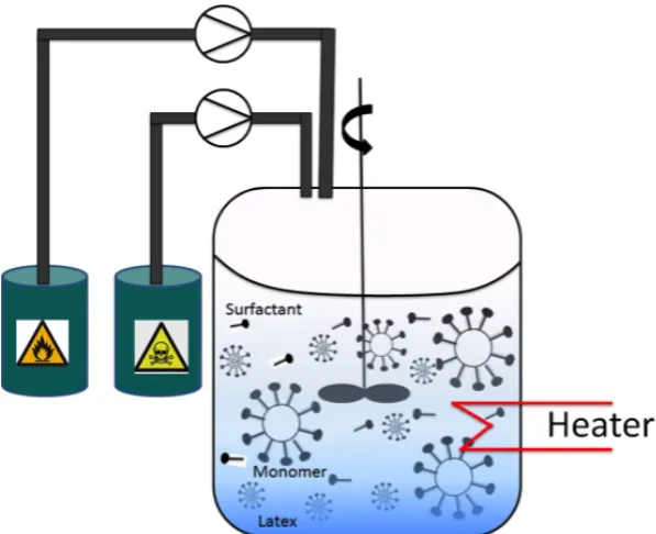
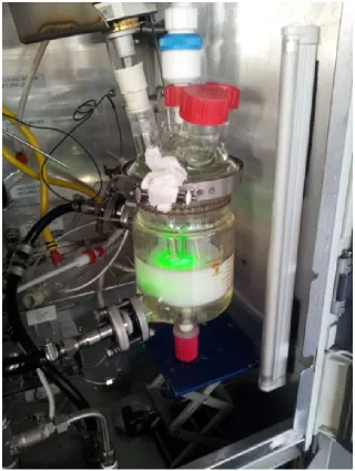
3.3.1 Experimental set up . . . 39
3.3.2 Adaptation of the MOAL algorithm . . . 43
3.4 Results and discussion . . . 46
3.5 Conclusions . . . 52
Chapter 4 Application of dimensionality reduction 53 4.1 Brief summary of the chapter . . . 53
4.2 Introduction . . . 53
4.3 Experimental . . . 56
4.3.1 Data sets . . . 56
4.4 Methods . . . 57
4.4.1 Dimensionality Reduction . . . 57
4.4.2 Classification in the reduced space . . . 62
4.5 Results and Discussion . . . 62
4.5.1 Visualisation . . . 62
4.5.2 Classification . . . 64
4.6 Conclusions . . . 70
Chapter 5 Concept development 72 5.1 Brief summary of the chapter . . . 72
5.2 Introduction . . . 73
5.3 Methods . . . 76
5.3.1 Expert systems based approach . . . 76
5.3.2 An evolution-based approach . . . 79
5.4 Merits and drawbacks of the proposed approaches . . . 81
Chapter 6 Discussion and Outlook 83
6.1 Conclusions . . . 86 6.2 Concluding remarks . . . 87
Appendix A Matlab code for the MOAL algorithm 88
Appendix B Matlab code for the extension of the MOAL algorithm 115
Appendix C Matlab code for categorisation of formulations as
Acknowledgments
There are several people to whom I wish to express my gratitude. I would like to
thank Professor Alexei Lapkin for his great supervision, support and encouragement
during this work. Your advice on both research as well as on my career have been
extremely useful. I would also like to thank Associate Professor Colm Connaughton
for being a great adviser. I would like to thank you for encouraging my research
and for allowing me to grow as a research scientist. I would like to express my
appreciation to Professor Evor Hines for fruitful discussions during my work. My
gratitude is extended to all members of the Reaction Engineering group at
Cam-bridge University for their help and support. Last but not least I would like to
express the warmest thank you to my girlfriend, Emma, for always backing me up
Declarations
I herewith declare that this thesis contains my own research performed under the
supervision of Professor Alexei Lapkin, without assistance of third parties. No part
of this thesis was previously submitted for a degree at any other university.
Material in chapter 2 is based on:
Peremezhney, N., Connaughton, C., Hines, E., Lapkin, A.A. (2013). Combining
Gaussian Processes, Mutual Information and a Genetic Algorithm for multi-target
optimization of expensive-to-evaluate functions. Engineering Optimization.
(Ac-cepted for publication).
Material in chapter 4 is based on:
Peremezhney, N., Connaughton, C., Unali, G., Hines, E., Lapkin, A.A. (2012).
Ap-plication of dimensionality reduction to visualisation of high-throughput data and
building of a classification model in formulated consumer product design. Chemical
Abstract
The research topic addressed in this thesis is the development of new ideas and
techniques for acceleration and automation of processes involved in the design of
chemical products with predefined properties. In particular, we demonstrate
tech-niques that address the shortcomings of the existing methods and take a bird’s-eye
view over the new possible directions for chemical product development necessitated
by the integration of bio-feedstocks into the existing supply chain. Furthermore, we
introduce an approach for sequential, on-line multi-target product/process
optimiza-tion in a scenario where: automaoptimiza-tion of the overall design process is sought; adequate
physical models are not available; unknown constraints on the decision space may
be present; and resources are limited or costly. We test the approach on a number of
simulations. The results indicate that the approach is able to, in a modest number
of iterations, find solutions associated with the targets to a satisfactory degree of
ac-curacy. In addition, for supervised problems where categorical data are available, we
introduce an approach that allows one to perform categorization of a given product
composition according to a particular property. We test our solutions empirically
on real data. The results show that the approach compares well with existing state
of the art techniques. We also investigate the application of a variety of nonlinear
Chapter 1
Introduction
The aim of chemical product design is to find a product that exhibits certain speci-fied behaviour/properties, corresponding to the desired functional properties. Thus,
in the area of chemical consumer products (sometimes termed formulated products)
the main useful functions, for example the function of ‘moisturising’ or the function of ‘UV protection’, are achieved through the use of molecules and particles with
the corresponding required physico-chemical properties, e.g., UV absorbance and
scattering of light by TiO2 particles, thus reducing the flux of the harmful range of
UV solar radiation to the skin. These main useful functions in consumer products
are accompanied by a varied cocktail of secondary desired functions, such as ‘feel’,
‘smell’, ‘colour’, etc. Various harmful functions could also be specified, which in-clude any side effects, the cost to the consumer, the cost to the manufacture and the
environmental impact of manufacture and use of the products. Traditionally, success
of the developed chemical consumer product relied on an engineer’s [formulator’s] experiential knowledge of what combinations of ingredients (formulations) work for
the required product application/s as well as the engineer being able to, through
random experimentation or via the use of statistical/machine learning techniques, find the composition of proportions of the identified ingredients that translate into
a product with predefined values/qualitative descriptions of the desired main and
secondary functional properties, e.g. transparency of 80%, high viscosity liquid, etc.
The demand for ‘green’ chemical products coupled with strong competition in the
market place, dictating shorter product-to-market times, is prompting the manufac-turers to update their ingredient libraries with molecules not previously used and
ap-proaches, based on mechanistic or empirical modelling, aimed at helping reduce the
costs associated with product development. The areas under scrutiny are: experi-mental design, process/predictive modelling, and optimization.
The needs of chemical product design dictate that the data driven methods involved deliver:
• Process models, physical or empirical, that are: capable of characterizing the effects of the interplay among product constituents on product properties.
• Design of experiments that reveal the most information about the underlying physical process.
• Target/global optimization approaches that can deal with multiple objectives.
1.1
Observations with regards to current state of affairs
1. Physical modelling involves constructing models based on the underlying physics
and chemistry governing the behaviour of the process. It bears high costs in terms of human effort and expertise, and can also be very time consuming. It
is, thus, rarely employed. Empirical modelling is carried out by considering
only the functions that belong to a restricted class or a number of classes, which may result in processes not being well modelled and, consequently, in
unsatisfactory approximations. Moreover, as experimental design is performed
in conjunction with the model that is to be fitted to the data, considering only a particular model class or classes bears direct consequence on the quality of
experimental designs and, subsequently, on the outcome of optimization.
2. There is a lack of data driven techniques addressing the scenario of multi-target
optimization in the presence of limited amount and/or high cost of materials.
3. There is a lack of real time multi-target optimization approaches where mod-elling, experimentation and optimization are part of a closed feed back based
loop.
1.1.1 Discussion of observation (1)
Successful design and optimization of a chemical product depends on the availability of adequate models relating composition of the product constituents to the
unavailable. Research and development efforts of chemical consumer product
man-ufacturers, however, are seldom concentrated to address this issue. The reason for it is that development of fundamental knowledge, being time consuming and
expen-sive in term of human expertise, is seldom justified, as research and development
costs are greatly influenced by a product’s short lifespan on the market [1]. The prevalent approach in the industry is to employ empirical modelling through the
use of Design Of Experiments (DOE) together with Response Surface Methodology
(RSM). DOE is a procedure for preparing experiments so that the data collected can be analysed to bring about valid conclusions. When chosen well, experimental
de-signs maximize the amount of ‘information’ that can be obtained with the planned
experiments. RSM is a group of mathematical/statistical techniques for building empirical models. The objectives are, using a chosen DOE, to optimize the output
variable (response), which is affected by a number of input variables, and to create
a predictive model of the relationship between the input variables and the response. A typical sequence of steps for an approach based on joint application of DOE and
RSM is:
1. Select a statistical model to approximate the response surface with and an optimization algorithm to drive the search for the optimum solution.
2. Given the model, employ a DOE method to choose a set of input configurations
for which the values of the output variable are to be obtained via interaction with the real system - the training set.
3. Use the training set to train and validate (through cross-validation) the
sta-tistical model.
4. Use the trained statistical model together with a chosen optimization
algo-rithm to predict the optimum solution.
The RSM-DOE based approaches are often made sequential by repeating steps 2 to 4 until a chosen stopping criteria is met. The training data set size is usually of
the order 10 times the number of the input variables. As obtaining a separate test
data set is often expensive,k-fold cross-validation is performed at model validation stage with the value of k chosen in the range between 10 and N (leave-one-out),
where N is the size of the available dataset. Models for response surface
approx-imation, presently most favoured by the industry, are Polynomial Regression and Artificial Neural Networks (ANNs). The main draw-back of employing polynomial
approximation is that modelling is carried out by considering only the functions that
not being well modelled and, consequently, in unsatisfactory approximations. Some
of the biggest shortcomings of ANNs are the lack of methodology for choosing the number of hidden layers (and the number of units in a hidden layer) and difficulties
associated with relating network weights to physical parameters [2]. In the work
presented in this thesis we apply Gaussian Process Regression (GPR) [35] for re-sponse surface approximation. This probabilistic non-parametric technique is truly
data driven, as it seeks the relationship among the observations, rather than trying
to approximate the modelled process by fitting the parameters of the selected ba-sis functions [4]. GPR based optimisation approaches have become a very popular
choice for global optimisation problems. However, research into theoretical
perfor-mance of GPR based optimization is still in it’s infancy [36]. Although RSM based techniques are currently a popular choice, non-model based direct search
optimisa-tion techniques such as the NelderMead simplex algorithm [13], for instance, have
also, historically, been employed in the industry.
1.1.2 Discussion of observation (2)
A frequently occurring situation in chemical product design is that of the limited
amount or high cost of materials. In this scenario it is possible that the training set obtained, whilst providing enough information to train a good predictive model,
may contain a high proportion of points that are not near the optimum, which would
lead to inefficient use of resources. Exploration of approaches that deal with the scenario of expensive function evaluations has recently received significant attention
in the research community. A number of approaches have been put forward that
have a common underlying scheme, namely, the idea of integrating the DOE into optimization [30; 33; 36; 7; 8; 37; 5; 6; 9; 10]. The key steps of such an approach
are:
1. Sample a small proportion of the allowable number of training points and train
the predictive model.
2. Approximate the response surface, select a solution that satisfies both the criteria for optimality of the DOE and the optimization problem in hand as a
whole. Evaluate the solution. If the optimum solution has been found, stop.
Otherwise, go to step 3.
3. Augment the training set, update the model and go to step 2.
GPR is particularly well suited for such sequential optimization. The variance of
space, whilst the mean predictions could be employed to give estimates of
prox-imity to the target or a measure of improvement on the current optimum if the optimization is global. Variants of a single-objective, sequential response surface
model based optimization approach have already been tried in the field of
chemi-cal reaction optimization. In [11], for instance, maximization of the trans-stilbene conversion rate in the epoxidation of trans-stilbene over Co2+-NaX catalyst is
per-formed to validate a sequential optimization approach based on RSM. The authors
utilise Gaussian Processes as the model for response surface approximation. At each iteration the mean and variance of the predicted observations are checked against
a predefined pair of mean and variance values through a set of inequalities, thus
guiding the search for the regions of the design space to be sampled in the next batch of experiments. Techniques for on-line sequentialmulti-target optimization of
chemical products/processes in the presence of limited amount and/or high cost of
materials, to our knowledge, are not currently available. In this thesis we present a technique for such optimization.
1.1.3 Discussion of observation (3)
At present, a hot research topic is the automation of chemical product/process development. To this end, there has been some success within the development
of ‘closed-loop’ micro-reactor systems that incorporate real-time experimentation,
statistical modelling and sequential DOE. By integrating sensors capable of reading off the output measurements and a computer program, running a machine learning
algorithm/s that accepts the sensor data and outputs information about a suggested
next experiment, within a continuous flow reactor, the automation of the overall reaction optimization is achieved. In [12] for instance, the authors present a
self-optimising micro-reactor system that employs the NelderMead Simplex algorithm
for optimization of a Heck Reaction. To our knowledge, an on-line sequential ‘closed-loop’ feedback integrated approach has not yet been applied formulti-targetchemical
product/process optimization.
1.2
Categorisation of product compositions
(formula-tions) and data visualisation
As well as exhibiting specified behaviour, corresponding to the desired main func-tional properties, a chemical consumer product has to be able to perform a number
Performance criteria for such functions is not easily quantifiable. In such instances
the output domain is no longer a set of continuous values, as in a regression case, but rather a set of categories, representing the spectrum of qualitative descriptions
of the desired secondary function. The task is then to first, design and evaluate a set
of experiments most informative about the location of the category boundary/ies, then, select and train a classification model capable of robustly predicting the
cat-egory of the desired function, given a particular formulation.
The kind of problems encountered in chemical product design are often
charac-terised by high dimensionality. Applying classification in these instances can cause
biased estimates [3], thus affecting the accuracy of predictions. It can also lead to high costs in terms of computation time [14]. To address these issues, in this thesis
we perform classification in the reduced space via application of a dimensionality
reduction technique. There are a number and a variety of techniques available for dimensionality reduction. The widely known and used ones are Principal
Compo-nent Analysis (PCA)[61] and multidimensional scaling (MDS)[62]. However, the
effectiveness of both PCA and MDS is limited by their global linearity. In order to resolve the problem of dimensionality reduction in nonlinear cases, the manifold
learning techniques such as locally linear embedding (LLE) [64] and Isomap [65], for instance, could be employed. Classification in the reduced space could be performed
by a simple technique such as ak-NN [72], for instance. It must be noted, however,
that for some highly non-linear problems where class separation is difficult (in the reduced space) it may be more appropriate to employ a probabilistic model such
as multinomial logistic regression or Gaussian process classification (GPC) [35] or
integrate fuzzy logic [60] into classification.
In this thesis we perform classification in the reduced space provided by a
non-linear supervised dimensionality reduction technique such as SIsomap [66]. To gain actionable insight, it is also important that the available evaluated data are
visu-alised. In this respect, unless the number of ingredients in a product is not higher
than three, it is also necessary to consider the employment of a dimensionality re-duction technique.
In this thesis we introduce an approach that incorporates dimensionality reduction as part of an algorithm for categorization of a given product composition according
to a particular property. We compare prediction results of this approach with
variety of non-linear dimensionality techniques to visualisation of chemical product
data.
1.3
Integration of bio-feedstocks and new possible
di-rections for consumer product development
At present the use of bio-feedstocks in consumer product design is relatively lim-ited, due to a small range of molecules available on the market, primarily natural
oils, flavour and fragrance substances, nutraceuticals, bio-pharmaceuticals. How-ever, this range is expected to be rapidly expanded, offering new opportunities for
product design. The emerging question is whether our existing methods of product
design in formulations and other chemistry using industries are appropriate for the new developing supply chain based on sustainable renewable feedstocks?
Our current approach to formulated product design is based on heuristic knowl-edge of formulators that allows selecting individual compounds from a library of
available materials with known properties. We speculate that most of the
com-pounds (or functions) that make-up the product to be designed can potentially be obtained from a single or very few bio-sources. In this case, it may be possible to
design a sequence of transformations required to transform feedstocks into products
with desired properties, analogous to a metabolic pathway of a complex organism. In this thesis, we conceptualise some novel approaches to processing bio-feedstocks
with the aim of bypassing the step of a fixed library of ingredients. Two approaches
are brought forward: one making use of knowledge-based expert systems and the other making use of applications of metabolic engineering and dynamic
combinato-rial chemistry.
This thesis contributes to the area of chemical product/process design and
optimi-sation. Specifically, it introduces novel techniques for multi-target product/process
optimization and categorization of a given product composition according to a par-ticular property. It also introduces novel ideas and concepts for acceleration and
automation of processes involved in the design of chemical products.
In summary, the objectives this thesis is addressing are:
1. Development of an approach for sequential, on-line multi-target
is sought; adequate physical models are not available; unknown constraints on
the decision space may be present; and resources are limited or costly.
2. Development of an approach that allows to perform categorization of a given product composition according to a particular property, for supervised
prob-lems where categorical data are available.
3. Development of new ideas and concepts for acceleration and automation of
processes involved in the design of chemical products with predefined
proper-ties.
The rest of the thesis is organised as follows. In Chapter 2 we present an approach for sequential on-line multi-target optimization in a scenario where: automation of
the overall design process is sought; adequate physical models are not available;
un-known constraints on the decision space may be present; and resources are limited or very costly. In chapter 3 we describe application of the approach presented in
chapter 2 to on-line multi-target optimization of a copolymerization reaction. In
Chapter 4 we introduce an approach that incorporates dimensionality reduction as part of an algorithm for categorization of a given product composition according
to a particular property. We compare prediction results of this approach with
sev-eral well-established classification models. In this chapter we also investigate the application of a variety of non-linear dimensionality techniques to visualisation of
formulated product data. In Chapter 5 we provide insight into and attempt to conceptualise new approaches to chemical product development. In particular, we
discuss the integration of expert systems, metabolic engineering and dynamic
com-binatorial chemistry in designing new ways of processing bio-feedstocks in chemical product design. Finally, in Chapter 6 we provide concluding remarks and consider
Chapter 2
Sequential Multi-Target
Optimization of
Expensive-to-Evaluate
Functions
2.1
Brief summary of the chapter
In this chapter a novel approach to multi-target optimization of expensive-to-evaluate functions is explored that is based on a combined application of Gaussian Processes,
Mutual Information and a Genetic Algorithm. The aim of the approach is to find
an approximation to the optimal solution (or the Pareto optimal solutions) within a small budget. The approach is shown to compare favourably with a surrogate based
on-line evolutionary algorithm on two synthetic problems.
2.2
Introduction
In target optimization one is concerned not with finding the global optimum (unless
the target happens to be one), but rather with finding solutions associated with
desired values of the underlying process/es. Such optimization problems often arise in product design. In particular, when novel materials and/or methods are involved,
it is usually required that certain desired specifications/properties of the product are adhered to. For example, in designing a formulated product such as facial cream
(using a constantly updated set of ingredients) it is important that certain
characteristics. In general, this poses a challenging engineering problem in that our
capacity to accurately predict properties of formulated consumer products based on composition is quite limited, due to the physical complexity of the system [34]. Our
ignorance about the underlying process leads to the need for an often large number
of interactions with the real system1. For some applications the number of interac-tions that can be performed is limited due to high cost of the resources involved.
In these instances an attractive strategy is to sequentially select experiments that
are optimal both in terms of experimental design and in terms of identification of suitable solution/s. The strategy is usually implemented via employment of a
surro-gate model for approximation of values of the response variable in combination with
a selective, one-at-a-time, sampling strategy where information from past experi-ments is used to determine the design of the next one. One of the most prominent
algorithms for such sequential optimization is Efficient Global Optimization (EGO)
[33]. Since its introduction, the algorithm has been adapted for different types of optimization problems, including target optimization. In [37], for instance, the
au-thors make use of the concepts of desirability [32] and virtual observations [28] to
construct an algorithm capable of identifying and, with each iteration, improving on a cluster of solutions that best associate with target values. Even though the
algorithm undoubtedly explores globally throughout the search, it is not designed to actively search for solutions that would allow one to gain the most information about
the underlying process (i.e. solutions optimal in terms of experimental design). In
this thesis a novel approach to sequential multi-target optimization is proposed that explicitly incorporates maximization of the information gain as one of its objectives.
Let x ∈ Rd; x ∈ Ω, were d is the dimension of the problem and Ω the decision
space, be the vector of values of the input variables, scalars y(x) and y∗ the
cor-responding observation obtained via interacting with the real system and a target
respectively, andXL={x1,x2, ...,xn} the set of candidate solutions (obtained via
discretization of the decision space). Then, for a single-target optimization, the
objective is to minimise the sum of regrets2
k
X
i=1
|y(xi)−y∗|, (2.1)
1
whereiis the iteration number, in other words to find
x∗= argmin
x∈XL
|y(x)−y∗| (2.2)
in as few iterations as possible. The cumulative regret, as in (2.1), i.e. the loss in
reward due to not knowing the points associated with the target beforehand, is a performance metric often used in this context [36]. Note, that the situation where
there are multiple solutions to (2.2) may arise. In this thesis we rank such
solu-tions using metric such as the hypervolume indicator [38], as explained further in the chapter. Alternatively, this scenario could be handled by the end user, ranking
the solutions by applying relevant cost functions. For instance, if the solutions are
compositions of ingredients in a formulation, then they can be further ranked in terms of cost of ingredients, or the proportion of a particular ingredient, etc.
The procedure for sequential single-target optimization in an expensive-to-evaluate function scenario could be:
1. Construct a cheap to evaluate surrogate model and train it on a sample of
points XT = {(x1;y(x1)),(x2;y(x2)), ...,(xh;y(xh))}, h n (the training
set).
2. Using the surrogate model’s predictions, selectx∗ that
• Maximizes information gain about the underlying process -exploration.
• Minimizes predicted regret, i.e. satisfies (2.2) -exploitation.
3. Evaluatex∗ via interacting with the real system and obtainy(x∗).
4. Include the pair (x∗, y(x∗)) in the training set and update the model.
5. Iterate until there is no improvement on the current optimum or the available
budget has expired. In the situation where the available budget has expired
prior to obtaining a satisfactory solution, the solution/s satisfying (2.2) is chosen from the solutions collected so far.
The above procedure requires that, at each iteration, two objectives are optimized
simultaneously. One way to go about it is to search for a set of non-dominated3 solutions - a Pareto set. A good way to select just one x∗ from a pareto set is to
choose a solution with the highest value ofhypervolume indicator. The hypervolume
3A solution is non-dominated if it cannot be superseded by another solution which improves an
indicator is the volume of the fitness space that is dominated by a solution4 and is
bounded by a reference point (see Figure 2.1). Also, the procedure entails choosing
x∗ from a predetermined decision set. Although practical in terms of computational
speed, this is limiting in terms of accuracy. It would, hence, be beneficial to find
a compromise between the increase in the level of discretization and the search of the entire decision space. The proposed compromise is to first, identify a set of
non-dominated solutions from a discrete set of candidate solutions, then, search in
the neighbourhood of these solutions, using a real-coded genetic algorithm (non-dominated sorting genetic algorithm II (NSGA-II) [29] is employed), for a solution
with the highest value of hypervolume indicator.
Industrial target optimization problems, however, often involve more than one
tar-get. For instance, a formulator may need to optimize a formulation for a particular
value of viscosity and opacity. The procedure described above can be extended to a multi-target case by constructing a separate surrogate model for each underlying
process and for x∗, replacing the values of information gain and regret associated
with it with chosen aggregates. In this thesis we use the magnitude of a vector whose entries are the values of information gain/regret as the aggregates. After the
termination of the multi-target optimization, all of the non-dominated solutions (in relation to the actual targets) could be identified and presented to the end user for
further consideration.
For the surrogate model, Gaussian Processes, as it provides a principled way of
assessing uncertainty of the model, has successfully been used in many
optimiza-tion problems and is the choice for the approach discussed here. As has already been mentioned, the sampling criterion is required to account for the need to both
exploit the knowledge acquired so far as well as gain more knowledge about the
underlying processes. The former can be achieved by choosing x∗ that, according to the surrogate model’s prediction will take us closer to the target, the latter can
be achieved, by choosingx∗ that is predicted to reduce the uncertainty about the
rest of the input space the most, which can be interpreted as the greatest increase in mutual information [31] betweenXT ∪x∗ and the rest of the input space.
Gaus-sian Processes allows us, through the use of the mean value (for the computation
of regret) and variance (for the computation of information gain) of the predicted distributions for the approximated underlying process values, to efficiently deal with
both demands on the sampling criterion.
4
0 0.2 0.4 0.6 0.8 1 1.2 0
0.2 0.4 0.6 0.8 1
f1
f2
R
P3 P2
[image:22.595.172.468.121.335.2]P1
Figure 2.1: The hypervolume (shaded area), bounded by a reference point R, of a three
point Pareto set{P1, P2, P3}. The hypervolume of pointP2 is the area of rectangle whose diagonally opposite corners areP2 andR.
The Efficient Global Optimization (EGO) algorithm would be, because of its suc-cessful application to optimisation problems, the best choice for comparison with
the approach proposed in this thesis. However, to our knowledge, there is no
suit-able adaptation of the EGO algorithm for multi-target optimisation. The approach proposed in this thesis is compared with a surrogate based on-line evolutionary
al-gorithm [30] that also uses Gaussian Processes. The alal-gorithm can easily tackle
multi-target optimisation problems. It should be noted that other surrogate based on-line evolutionary algorithms exist that are similar in their approach (see, for
in-stance, [40] and [41]). The attractive features of these algorithms are: they have
an evolutionary algorithm at the core, capable of solving dimensional, multi-modal problems; they attempt to strike a balance between the need to reduce the
amount of expensive evaluations and the need to improve on the quality of the
surrogate model. Although both, the approach presented in this work and the al-gorithm it is compared with, use Gaussian Processes, its application is different,
which makes for an interesting comparison. In the rest of the chapter, the
The chapter is organized as follows. In section 2.3, Gaussian Processes and Mu-tual Information are, briefly, introduced, followed by a description of the MOAL
algorithm in section 2.4. In section 2.5, we describe the application of the MOAL
algorithm to two synthetic multi-target optimization problems. In section 2.6 we, briefly, introduce the SOEA algorithm and describe its application to the synthetic
multi-target optimization problems. The results are discussed in section 2.7. In
section 2.8, we describe an adjustment of the MOAL algorithm for problems that involve unknown constraints on the decision space. Conclusions are drawn in section
2.9.
2.3
Methods
2.3.1 Gaussian Processes Regression
The assumption is that the observations associated with the inputs to the system
have a (multivariate) Gaussian joint distribution. Here, a random variable is an observation associated with a particular input. For any subset of the random
vari-ables, their joint distribution will also be Gaussian. A Gaussian Process (GP) is a
generalization of multivariate Gaussians to an infinite number of random variables. According to a GP definition, the joint distribution over observations associated
with every finite subset of inputs is Gaussian. These joint distributions are defined
by a GP through the use of mean function,m(·), and covariance function,k(·,·). For an observation associated with inputxits mean is given by m(x) and for a pair of
observationsxandx0 their covariance,K(x,x0), is given byk(x,x0). In this thesis
we consider stationary covariance functions. A stationary covariance function is a function ofx−x0. It is therefore invariant to translations in the input space. A
com-mon choice is to apply a Gaussian Process with zero mean function and Automatic
Relevance Determination (ARD) Squared Exponential covariance function
k(x,x0) =σ2fexp
− 1 2
D
X
d=1
xd−x
0
d
ld
!2
(2.3)
In the above,σf2 is the signal variance,ld is an individual characteristic length scale
for each input dimension xd. However, it is sensible to assume measurement noise
underlying processf(x) through a Gaussian noise model:
y(x) =f(x) +, (2.4)
were ∼ N(0, σ2n) are independent identically distributed (IID) random errors.
And so, the final expression for the covariance function - the prior on the noisy
observations can be written as
kf inal(x,x
0
) =σ2fexp − 1 2 D X d=1
xd−x
0
d
ld
!2
+δxx0σn2, (2.5)
were δxx0 is the Kronecker delta function. θ = n
σ2f, l1, l2, ..., ld, σn2
o
forms a set
of hyperparameters of the covariance function. To incorporate the knowledge that the training data provide about the process we write the joint distribution of the
observed target values and function values at test locations under the prior and then
condition it on the observations. The necessary Gaussian identities employed are:
" x y # ∼ N " µx µy # , " A C
CT B
#! ,
werexand yare jointly Gaussian random vectors; and the marginal distribution of
xtogether with the conditional distribution ofx giveny
x∼ N(µx, A),
x|y∼ N µx+CB−1 y−µy
, A−CB−1CT .
So, now, given a set of inputs to the system,X, corresponding observations,y, and an unobserved inputx∗, fory(x∗)
" y
y(x∗) #
∼ N 0, "
K(X, X) K(X,x∗)
K(x∗, X) K(x∗,x∗) #!
, (2.6)
where each entry in K(·,·) is computed using (2.5). The conditional probability,
P(y(x∗)|y), then follows a Gaussian distribution:
The mean and variance of this distribution are used to compute the best estimate
and the uncertainty ofy(x∗):
¯
y(x∗) =K(x∗, X)K(X, X)−1y, (2.7)
σy2(x∗)=K(x∗,x∗)−K(x∗, X)K(X, X)−1K(X,x∗). (2.8)
A number of models can be constructed depending on the choice of the values of
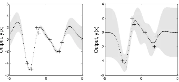
the hyperparameters in the covariance function. Figure 2.2 illustrates two output
vectors where the mean and variance of each output have been computed using (2.7) and (2.8), but where the values of the hyperparameters of the covariance function
are different. To choose the best model for the data available, a search is carried
out for the values of the hyperparameters that maximize the marginal likelihood -the probability of -the data given -the hyperparameters,
logp(y|X,θ) =−1 2y
TK−1y−1
2log|K| − n 2log 2π,
where|K|is a determinant of matrixK and nis the number of training examples.
As the mean function is set to 0, it’s values do not appear in the expression of the marginal likelihood. To set the hyperparameters, partial derivatives of the marginal
likelihood w.r.t. the hyperparameters are obtained and used in conjunction with a
gradient based optimizer. The advantage of using marginal likelihood is that it au-tomatically incorporates a trade-off between model fit and model complexity. Note,
that in order to account for uncertainty in the hyperparameters, integration over
the posterior distribution of the hyperparameters is required. The integral over the posterior of the hyperparameters often is not analytically tractable, though. A
com-monly employed approach is to use numerical integration via Markov chain Monte
Carlo (MCMC)-methods. But, due to the computational burden, this approach may be too costly for large data sets. To train a GP model, a choice has to be made
(utilizing prior knowledge) between different functional forms for the mean and
co-variance functions as well as adaptation of the hyperparameters of these functions. In the absence of prior knowledge, a variety of functional forms could be investigated
via comparison of the marginal likelihoods (for more details see [35]). In this thesis,
only GP with zero mean function and Squared Exponential (ARD) covariance func-tion and GP with zero mean funcfunc-tion and Mat´ern covariance function, as described
Figure 2.2: Two output vectors where the mean and variance of each output have been computed using (2.7) and (2.8), but where the values of the hyperparameters of the co-variance function are different. The training data are shown by + signs. The output predictions (dots) were generated using a GP with the covariance function as in (2.5) with: left - (l, σf, σn) = (1, 1, 0.1); right - (l, σf, σn) = (
√
3,0.5,0.8). Both plots also show the 2 standard-deviation error bars for the predictions obtained using these values of the hyperparameters.
2.3.2 Mutual Information
Mutual information of two random variablesXand Y measures how much knowing
one of these variables reduces uncertainty about the other. It is expressed as
M I(X;Y) =H(X)−H(X|Y), (2.9)
wereH(X) is a marginal entropy - the amount of uncertainty about random variable
X and H(X |Y) is a conditional entropy - the amount of uncertainty remaining aboutX afterY is known, computed as
H(X|Y) =H(X, Y)−H(Y). (2.10)
The above gives support to the intuition behind the meaning of mutual information as the reduction in uncertainty that knowing one variable provides about the other.
Mutual information is non-negative and symmetric. Namely,
M I(X;Y)≥0 (2.11)
and
For a random variableX with a probability density functionf whose support set is
X, the differential entropy H(X) is defined as
H(X) =− Z
X
f(x) logf(x)d(x). (2.12)
The differential entropy of a Gaussian random variableX conditioned on variable Y is a monotonic function of its variance:
H(X|Y) = 1 2log
2πexpσ2X|Y. (2.13)
If X is assumed to be an observation associated with a particular input to the system as discussed in the previous section, for instance, then, using GP regression,
predicted value of σX|Y2 is easily computed using (2.8). Also, as the computation
in (2.8) only depends on the inputs, it is possible to compute H(X|Y) before the actual observation is made. It is useful, in the context of optimization, to think
of a discretized input space as a set of random variables. Let XL be such a set of
random variables,XT be any subset ofXLand x any random variable inXL\XT,
then the mutual informationM I(XL\XT ∪x;XT ∪x), expressed as
M I(XL\XT ∪x;XT ∪x) =H(XL\XT ∪x)−H(XL\XT ∪x|XT ∪x),
is the information gain (or the amount of uncertainty remaining aboutXL\XT∪x
(the rest of the input space)), ifxis revealed.
2.4
MOAL algorithm
We assume the underlying physical processes are unknown. The experimental data
(real observations) are used to train the surrogate models that approximate the un-derlying unknown physical processes.
Consider n objectives, associated with n targets, as in (2.2), and a budget of t evaluations. Two sets of points are involved: the training set, XT, which is used
to train the surrogate models and which gains a point with each iteration of the
algorithm; and a set, XL, of other solutions from a discretised decision space. A
surrogate model is trained for each process. Then at each iteration of the algorithm:
1. Using the surrogate models, estimates and the associated predicted variances
2. In relation toi’s objective, every point is referenced in two ways:
(a) The increase in mutual information it would provide [31]:
I(i)(xj) =M I(XT ∪xj;XL\XT ∪xj)−M I(XT;XL\XT) (2.14)
=H(XT ∪xj)−H(XT ∪xj |XL\XT ∪xj)
−[H(XT)−H(XT |XL\XT)]
=H(XT ∪xj)−H(XT)
−H(XT ∪xj |XL\XT ∪xj) +H(XT |XL\XT)
=H(xj |XT)−[H(XL)−H(XL\XT ∪xj)]
+H(XL)−H(XL\XT)
=H(xj |XT)−[H(XL\XT)−H(XL\XT ∪xj)]
=H(xj |XT)−H(xj |XL\XT ∪xj)
= 1
2log 2πeσ
2(i) (xj|XT)−
1
2log 2πeσ
2(i)
(xj|XL\XT∪xj)
= 1 2log
σ2((ix)
j|XT)
σ2(i)
(xj|XL\XT∪xj)
where (2.9), (2.10) and (2.13) are employed to write H(XT ∪xj) −
H(XT) asH(xj |XT),H(XT ∪xj |XL\XT ∪xj) asH(XL)−H(XL\XT ∪xj),
H(XT |XL\XT) as H(XL)−H(XL\XT) and equation (2.8) is used
to computeσ2(i)
(xj|XT) and σ
2(i)
(xj|XL\XT∪xj).
(b) The predicted value of regret
r(i)(xj) =|y¯(i)(xj)−y∗(i)|, (2.15)
where ¯y(i)(xj) and y∗(i) are the predicted value of the response variable
iatxj and the target value of the response variable irespectively.
3. The setsI(i)(x
1),I(i)(x2), ...,I(i)(x|XL|) and
r(i)(x1), r(i)(x2), ..., r(i)(x|XL|)
summarized as
I(xj) =
I(1)(x
j)
I(2)(x
j)
... I(n)(x
j)
, r(xj) =
r(1)(xj)
r(2)(x
j)
...
r(n)(xj)
, (2.16)
then, the magnitudes kI(xj)k2 and kr(xj)k2 are computed. The following
procedure5 is then used to choose one point for sampling:
(a) All of the points are sorted according to non-domination, using the
mag-nitudeskI(xj)k2andkr(xj)k2, and a Pareto set,χ, identified. The point,
xc, satisfying
xc= argmax
xj
kI(xj)k2×
√
n− kr(xj)k2
(2.17)
is chosen as the ‘current best’. Set χ is, first, reduced to size z |XL|
(to include onlyxc and at most z−1 ‘next best’ non-dominated points
selected according to (2.17)) and, then, used as the first population for a NSGA-II algorithm (without crossover) to conduct a search for the
maximizer.
(b) The NSGA-II algorithm is iteratedM times. At each iteration:
• Following sorting and selection steps, mutations are carried out (by performing small perturbations of the input vectors) to obtain a set (of size|χ|) of new points within the decision space.
• Each of the new points is referenced using (2.14) and (2.15) and one point is chosen according to (2.17). If the value computed for it using (2.17) is higher than that one of the ‘current best’ point, it becomes
the ‘current best’ point.
• The ‘current best’ point after the M th iteration is chosen for evalu-ation.
4. The evaluated point is added to the training set and the hyperparameters of
the surrogate models are reoptimized.
Note that for points in XL that are near the one that was just sampled their
pre-dicted variance,σ2(x
j|XT) (see last line in equation (2.14)) will decrease, as will the
5
associated value of the increase in mutual information. This means that,
poten-tially, the points close to the target will not be sampled for a number of iterations. To overcome this problem, the decision set XL is re-sampled with density ˆpXL∗|x˜
(where x˜ is a matrix of solutions collected so far), when there has been no
im-provement in the value of the hypervolume indicator of the Pareto set for a num-ber6 of consecutive iterations. Re-sampling with ˆpX∗
L|x˜ is done using a mixture of
Gaussians (with n components) as a density estimator. The value of the
hyper-volume indicator of the Pareto set is obtained as follows: first, the observations n
y1(1), ..., y1(n);y(1)2 , ..., y2(n);...;ym(1), ..., ym(n)
o
, collected so far, are transformed as
|yj(i)−y∗(i)|
R(i) , i= 1, ..., n j= 1, ..., m (2.18)
where
R(i)= max|yj(i)−y∗(i)|; (2.19)
then, from the transformed observations, the non-dominated set is identified and
the value of the hypervolume indicator (for the whole of the non-dominated set), bounded by a reference point, which is a vector of ones and of lengthm, computed.
As discussed above, relevant to the accuracy of the algorithm, the signal for the resampling of the decision set could be when there has been no improvement in the
value of the hypervolume indicator of the Pareto set for a number of iterations. The
same could be applied as a stopping criteria for the overall algorithm. However, there is danger of stopping too early. Instead (or additionally) the algorithm could
be stopped ones a solution is found that is within an acceptable error away from the
target. However, there is no guarantee that solutions within the predefined error ex-ist, in which case there is danger of performing more experiments than necessary. In
this thesis, for the lack of a robust error based stopping rule, we stop the algorithm
once the budget of evaluations is exhausted. The final Pareto set is presented to the end user. For comparison of performance against other algorithms (or against
op-timum performance, if such information is available), the value of the hypervolume
indicator for the final Pareto set (bounded by a reference point, which is a vector of ones and of lengthm) can also be computed. To reduce computational complexity,
σ2((ix)
j|XL\xj) is calculated using onlyk points, where
2|XT| ≤k≤ |XL\xj|. (2.20)
6
Namely, points x0 ∈ XL\xj are arranged in decreasing order according to their
respective values of covariance with xj (computed using (2.5)) and the first k are
selected.
It should be noted that, although presented specifically as a multi-target optimiza-tion algorithm, MOAL can still be applied in situaoptimiza-tions where some objectives are
global. In such cases all that is required is a suitable ‘unreachable’ target. For
in-stance, if minimization of monetary cost is one of the objectives, it can be converted into a target of£0.00. In chapter 3 an optimization problem with one target and
one global objective is discussed.
2.5
Illustration of the approach
To illustrate the potential use of the approach, it is applied to simulate two
multi-target optimization problems. The Ackley [42], the Booth [43], the Levy [44] and the Dixon & Price [45] functions where employed to simulate fictitious physical
pro-cesses. These functions are widely used for testing optimization algorithms. The first
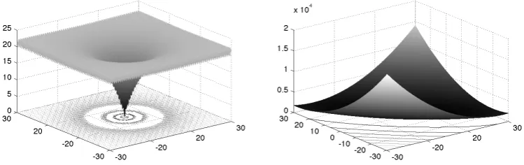
problem illustrates the application of the algorithm to a two-target unconstrained optimization problem, where: the two fictitious physical processes are simulated by
[image:31.595.136.511.455.573.2]the Ackley and the Booth functions (see Figure 2.3)
Figure 2.3: Left: the Ackley and right: the Booth functions in two dimensions.
fAckley(x, y) = − 20 exp
−0.2p0.5 (x2+y2) (2.21)
− exp (0.5 (cos (2πx) + cos (2πy))) + 20 + exp (1),
fBooth(x, y) = (x+ 2y−7)2+ (2x+y−5)2, (2.22)
where fmin(1,3) = 0;
the number of input variables is two, with each one ranging from −30 to 30; and
both targets are global minimums. Thus, the target vector is [0 0]T. The set of candidate solutions,XL, comprises of 1200 input vectors uniformly spread out over
the decision space. The initial training set, XT, comprises of 16 input vectors,
obtained as a Latin Hyper Cube (LHC) [46] sample, and corresponding values of two processes. The values of the Booth function are log transformed prior to regression.
For this problem a GP with zero mean and the Mat´ern covariance function was
employed
kMat´ern
x,x0=σf2 2
1−νΓ (ν) √ 2νr l !ν Kν √ 2νr l ! , (2.23)
with positive parametersν,σ2f and l, where Kν is a modified Bessel function and
r=|x−x0|. ν = 32 was chosen for this problem, for which (2.23) can be simplified
[27] to
kMat´ern
x,x0=σf2 1 + √ 3r l ! exp − √ 3r l ! . (2.24)
The parameters σ2f and l in (2.23) and (2.24) play the same role as in (2.3). Note, there is just one length parameter, as opposed to one per dimension of the problem.
The first problem is challenging as, in order to approximate the optimal Pareto set well, the algorithm is required to find solutions that are near both global
min-ima. A big proportion of the landscape of the Ackley function is featureless, thus, a
surrogate model trained on a small initial training set may not be able to produce satisfactory predictions for points in the target area, and the algorithm will need
to explore efficiently (i.e. update the surrogate model with most informative points quickly), for an optimization to converge on a satisfactory set of solutions within a
small budget of evaluations. For the Booth function, the global optimum is inside
a long, flat valley. To find the valley is not difficult, however, convergence to the global optimum is challenging. For the Ackley function, the global optimum is inside
a narrow funnel, making it also non-trivial to locate.
The second problem illustrates the application of the algorithm to a two-target
simulated by the Levy and the Dixon & Price functions
fLevy(x) = sin2(πy1) +
n−1
X
i=1
(yi−1)2
1 + 10 sin2(πyi+1)
+ (yn−1)2, (2.25)
were
yi= 1 +
xi−1
4 ,
fDixonPrice(x) = (xi−1)2+ n
X
i=2
i 2x2i −xi−1
2
; (2.26)
To mimic problems encountered in formulation industry where the problems are of-ten moderate dimensional, we set the number of input variables to four. A constraint
often encountered in industrial applications is also applied
4
X
i=1
xi =T, (2.27)
werexi∈R≥0 andT is user defined (T = 10 is used for this problem). The situation
is often encountered in experiments with formulated products, for instance, where
xi are volumes of ingredients andT is the total volume per formulation. Three
ran-dom target vectors were chosen from the h
fmin(1) (x), fmax(1) (x)
i
×hfmin(2) (x), fmax(2) (x)
i
box. The set of feasible solutions,XL, comprises of 2000 uniformly spread out
in-put vectors satisfying (2.27). The initial training set,XT, comprises of 30 uniformly
spread out feasible input vectors and corresponding values of two processes. For this problem a GP with zero mean and Squared Exponential (ARD) covariance function
was employed.
For both problems:
• Process values are perturbed by noise drawn fromN(0,0.12)
• In (2.20),k= 2|XT|is used
• The NSGA-II algorithm is iterated 100 times per iteration of the main al-gorithm with a population size at most 1% of|XL|. For each mutation, the
value of the perturbation is drawn from the uniform distribution on the inter-val (0, α60] and (0, α10] for the first and second problem respectively. Values of
the parameterαfrom the interval [0.01,0.1] were tested andα= 0.01 selected.
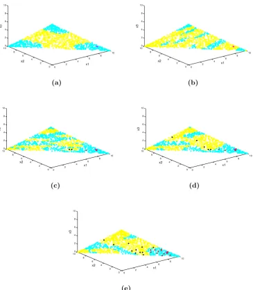
only the solutions so far collected, Xx∗, are considered. Xx∗ are assumed to
belong to a mixture of Gaussian distributions with the number of components that of the dimension of the input space. A Gaussian mixture model is
fit-ted [26] and the parameter estimates (components’ means, covariances and
mixture proportions) are obtained using an Expectation Maximization (EM) algorithm. A set of random input vectorsXL∗ (of the same cardinality asXL)
is then drawn from the resulting distribution.
The hyperparameters7 of surrogate models are fitted by optimizing the marginal
likelihood using a conjugate gradient optimizer. To avoid bad local minima 5 random restarts are tried, picking the run with the best marginal likelihood. Leave-one-out
cross-validation is used to validate the models. Namely, for each point in the training
set, its predicted function value along with the variance of the predicted value are computed using the rest of the set. Following [33], cross-validated standardized
residuals,Sr, are computed
Srx =
y(x)−y¯(x) q
σ2
y(x)
, (2.28)
and a check is carried out that the standardized residuals are all in the interval
[−3,+3]. When training surrogate models in problem 1, some of the computed standardized residuals failed the test. In an attempt to improve the fit of the
GPR models we log transformed the values of both the Ackley and the Booth
functions. The log transformation worked well and the standardized residuals where all inside the interval [−3,+3]. In general, if the GPR model fails the validation test,
we would try two transformations: the log transformation, log(y), and the inverse
transformation, −1/y. If this does not help, we would investigate the possibility of using a non-stationary covariance function. The optimizations are run for 30
iterations. The observations thus collected are transformed using (2.18). From the
transformed observations, the non-dominated set is identified and the value of the hypervolume indicator for the whole of the set (bounded by a reference point [1,1])
computed. The value is then compared against the one computed for the SOEA
algorithm and the optimum or a suitably chosen baseline. In this thesis, a baseline is obtained by computing the value of the hypervolume indicator for non-dominated
observations obtained having evaluated 10000 uniformly spread out input vectors.
7
2.6
Brief description of the SOEA algorithm for
multi-target optimization
In this work the approach proposed by [30] is adapted. The attractive features of this approach are: it has an evolutionary algorithm at the core, capable of solving
multi-dimensional multi-modal optimisation problems; it attempt to strike a
bal-ance between the need to reduce the amount of expensive evaluations and the need to improve on the quality of the surrogate model. Essentially, each iteration of the
approach consists of two steps: the search step and the function evaluation step. The search step involves the use of selection, crossover and mutation operators to
create a new population of solutions, promising in terms of proximity to the target.
The function evaluation step involves the use of a GPR model for approximation of the function values associated with each new population of solutions and
identifi-cation of solutions (within the new population) that need to be evaluated via real
experiments.
The SOEA algorithm proceeds as follows:
1. The initial population of solutions of sizeN is chosen. The initial population
of solutions and the corresponding observations are used as a training set to train surrogate models.
2. A GP with zero mean and Squared Exponential (ARD) covariance function is used. The surrogate models’ set up, validation and hyperparameter
optimiza-tion follows that described in secoptimiza-tion 2.5.
3. Using a multi-objective evolutionary algorithm (NSGA-II), the next
popula-tion of solupopula-tions is obtained.
4. The trained surrogate models are used to predict the mean values and the corresponding variances of the process values (see equations (2.7) and (2.8)))
for each of the obtained solutions. From the predicted variances of the process
values, corresponding standard deviations are computed and normalized to be in the interval [0,1].
5. Solutions for which the normalized standard deviation of each predicted
pro-cess value is below the currently allowable tolerance, Tolerancec, are assigned
The value of Tolerancecis updated after each iteration of the overall algorithm.
It is reduced as follows:
Tolerance(ci) = Tolerancem×
t−Total(si−1)
t−N , (2.29)
where Tolerancem is the maximum allowable tolerance (initialized prior to
optimization),tis the maximum number of interactions with the real system that are budgeted for, Total(si−1) is the total number of solutions (up to the
iterationi−1) that were evaluated via interacting with the real system, and
N is the number of solutions in a population. Prior to the first iteration, Tolerancec is equal to Tolerancem. To avoid an infinite loop scenario, where
evaluations are carried out using the surrogate models only, Tolerancem is
reduced by half if, at ith iteration all of the solutions in the population have been assigned their predicted values.
6. The hyperparameters of the surrogate models are reoptimized after each
iter-ation. The overall algorithm is iterated until the budget is exhausted.
Once the budget of evaluations has been exhausted, the algorithm is stopped. The
corresponding observations are transformed using (2.18). From the transformed
observations, the non-dominated set is identified and the value of the hypervolume (using ([1,1] as a reference point) computed. The same decision set and the initial
training set as for the MOAL algorithm where used. The initial value of Tolerancem
(i.e. the initial maximum allowable normalised standard deviation for the predicted process values) parameter was established through experimentation. Values between
0.05 and 0.5 were tested and a value of 0.1 selected.
2.7
Results and Discussion
The MOAL and SOEA algorithms were tested on the problems presented in section
2.5. Ten optimization runs were performed for each target vector and the mean
values of the hypervolume indicator of the Pareto set, along with corresponding standard deviations, were recorded (see Tables 2.1 and 2.2). These values were used
to compare the performance of the algorithms. For both algorithms theR(i)in (2.18)
were computed8 using observations from 10000 uniformly spread out solutions. As can be seen from the results, the MOAL algorithm has performed better than the
SOEA on both problems. The plausible explanation is that the MOAL algorithm is
8In real application these values would be established using all available observations after the
MOAL SOEA Baseline
[image:37.595.188.391.107.144.2]49.43%(4.11) 27.55%(15.86) 64.66%
Table 2.1: Mean and standard deviation of the hypervolume indicator of the Pareto set for
the target vector in problem 1 (after 10 runs of the algorithms). The Baseline column refers to the value of the hypervolume indicator of the non-dominated observations obtained by evaluating 10000 uniformly spread out input vectors.
MOAL SOEA Optimum/Baseline
Target vector 1 98.44%(0.68) 91.71%(3.90) 100% Target vector 2 87.01%(3.31) 81.98%(4.00) 93.12% Target vector 3 97.92%(0.50) 91.84%(1.78) 100%
Table 2.2: Mean and standard deviation of the hypervolume indicator of the Pareto set for
the target vectors in problem 2 (after 10 runs of the algorithms). The Baseline column refers to the values of the hypervolume indicator of the non-dominated observations obtained by evaluating 10000 uniformly spread out input vectors.
able toactively improve on the prediction quality of the surrogate models over the
target area, and do so rapidly (see Figure 2.4). Locating the areas of the decision space least well covered by the training set, whilst at the same time ‘promising’ in
terms of gaining on the targets, allows the MOAL algorithm to efficiently discover
relevant (for the optimization) features of the underlying function landscape. By contrast, the SOEA algorithm is only concerned with reducing uncertainty in the
search areas. In a situation where the underlying function landscape is challenging
and the budget of the evaluations is small the algorithm can be very successful or unsuccessful depending on how quickly the evolutionary part of it can converge on
solutions near the target area/s. This is reflected in the high value of the standard
deviation of the hypervolume indicator for problem 1 (see table 2.1).
The following performance criteria can be used to assess the quality of predictions
of the surrogate models:
1. Standardized9 mean squared error (SMSE) loss, which is the mean squared
error (MSE) normalized by the variance of the targets of the test cases.
2. The negative log probability (NLP) of the target under the model (since we produce a predictive distribution at each test input),
−logp(y∗|XT,x∗) =
1
2log 2πσ
2
∗
+(y∗−y¯(x∗))
2
2σ2
∗
, (2.30)
9
[image:37.595.140.478.213.280.2]−30 −20 −10 0 10 20 30 −30
−20 −10 0 10 20 30
−30 −20 −10 0 10 20 30
[image:38.595.124.517.109.268.2]−30 −20 −10 0 10 20 30
Figure 2.4: Contour plot of the Booth function with, left: input locations of the initial
training set and, right: solutions obtained using the MOAL algorithm for an optimization run of 30 evaluations. Empty squares - solutions from the initial training set; filled triangles - solutions chosen by the MOAL algorithm; squares with a cross inside - the global minima of the Booth and the Ackley functions.
where ¯y(x∗) and σ2∗ are the estimated mean and variance of the predictive
distribution respectively. This can be summarized by the mean negative log probability (MNLP), by averaging over the test set. This loss can be
standard-ized by computing it relative to the NLP of a predictive model that ignores the
inputs and always predicts using a Gaussian distribution with the mean and variance of the training data. The MNLP will, then, be approximately zero
for a simple predictive model and negative for a better one. Prediction quality of the surrogate models approximating the Booth function (as in problem 1)
is used as an example (see Figures 2.5 and 2.6). The test set is chosen to be
the solutions in and around the target area in the ([−5,5]×[−5,5] box).
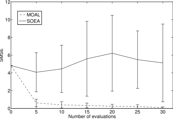
As can be seen from Figure 2.5, the surrogate models employed to approximate the Booth function during optimization runs of the MOAL algorithm, produced
predic-tions with smaller errors, on average. There is a big drop in the value of SMSE after
just 5 evaluations, and steady decrease thereafter, which indicates that the target area was found quickly, and that solutions are being chosen from it (the target area).
The MNLP value (see Figure 2.6) also decreases rapidly by 5 evaluations, although the improvement is less pronounced thereafter. It can be argued that for the SOEA
algorithm, on average, 30 evaluations were not enough to narrow down the search
and, hence, adequately update its surrogate models.
0 5 10 15 20 25 30 0
2 4 6 8 10 12
Number of evaluations
SMSE
MOAL
[image:39.595.150.445.132.335.2]SOEA
Figure 2.5: Average SMSE values computed for surrogate models approximating the Booth
function in problem 1. The averages were computed over 10 optimization runs for budget sizes from 5 to 30 evaluations in increments of 5. Zero evaluations corresponds to the values computed for the model constructed using the initial training set.
0 5 10 15 20 25 30
−5 0 5 10 15
SNLP (MOAL)
0 5 10 15 20 25 30
−10 0 10 20
Number of evaluations
SNLP (SOEA)
Figure 2.6: Average MNLP values computed for surrogate models approximating the
[image:39.595.149.449.441.643.2]