Localization of structural flaws in concrete sewer pipes by physical interaction inspection with a robotic arm

Localization of structural flaws in concrete sewer pipes by

physical interaction inspection with a robotic arm

E.J. (Edwin) van Boven

MSc Report

Committee:

H. Noshahri, MSc

Dr.ir. D. Dresscher

Prof.dr.ir. G.J.M. Krijnen

Dr.ir. L.L. Olde Scholtenhuis

May 2019

017RAM2019

Robotics and Mechatronics

EE-Math-CS

University of Twente

Contents

1 Introduction 1

1.1 Problem context . . . 1

1.2 Problem statement . . . 1

1.3 Research goal . . . 2

1.4 Research questions . . . 2

1.5 Outline . . . 2

2 Analysis 3 2.1 Structural flaws in sewer pipes . . . 3

2.2 Relation between material properties and structural flaws . . . 8

2.3 Rebound principle of assessing concrete . . . 13

2.4 Robotic assessment of concrete based on the rebound principle . . . 22

2.5 Conclusion of analysis . . . 25

3 Experimental Study 27 3.1 Design of experimental setup . . . 27

3.2 Description of experiments . . . 36

3.3 Validation of impact test . . . 38

3.4 Influence of internal deflection of the robotic arm on measurements . . . 42

3.5 Influence of spring settings on impact measurements . . . 48

3.6 Influence of elastic modulus on impact measurement . . . 51

3.7 Localization of flaws . . . 55

3.8 Discussion of experimental study . . . 59

4 Conclusion and recommendations 60 4.1 Conclusion . . . 60

4.2 Discussion . . . 61

4.3 Recommendations . . . 61

A Appendix Franka Emika Panda arm 63

1 Introduction

This report studies the feasibility of locating structural flaws in concrete pipes due to interac-tion with a robotic arm. In this chapter the context of this research is given, the problem is stated and the goal of this research is given. Also the research question is stated and divided into sub-questions. At the end of this section, the outline of this report is given.

1.1 Problem context

The origin of this research lays within the TISCALI project (NWO, 2017), which is an abbrevia-tion for ‘Technology Innovaabbrevia-tion for Sewer Condiabbrevia-tion Assessment - Long-distance Informaabbrevia-tion- Information-system‘. This project focuses on automation and information distribution of sewer pipe in-spection. An overview of the TISCALI project is given in figure 1.1.

Figure 1.1:Overview of Tiscali Project (RAM, 2019)

In the overview the different aspects of the TISCALI project are shown. One can see the zep-pelin, which represents inspection from higher altitude, in order to locate potential flaws in sewer pipe system. Another aspect shown, is a kind of sweeper on ground level. This repre-sents inspection of the sewer pipes from ground level with ground-penetrating radar. Which is used to locate structural flaws more precisely, based on the information retrieved from high altitude inspection. In case a certain pipe has a potential flaw, in-pipe inspection is required in order to locate the exact position and the severity of the flaw. This is represented with the cart that is shown inside of the pipe. This research is part of the research done by the TISCALI project that is focused on automation of in-pipe sewer inspection.

1.2 Problem statement

1.3 Research goal

The research described in this report covers the investigation of the feasibility of inspecting concrete with physical interaction. The physical inspection can be done in a variety of ways, but because time is limited, this research is only focused on physical interaction inspection with a robotic arm. The goal of this research is to determine if it is feasible to locate structural flaws in a sewer pipe by physically interacting with a robotic arm.

1.4 Research questions

As the goal is to study the feasibility of locating structural flaws by physically interacting with a robotic arm, the research question is formulated as following’To what extend can interaction between a robotic arm and the surface of a concrete pipe be used to locate structural flaws of the pipe?’

In order to give a structured answer on the research question, the question is divided into sub-questions. First it is important to determine which structural flaws occur in sewer pipes and which should be prioritized for location by physical interaction inspection. Which leads to the first subquestion:Which structural flaws in sewer pipes can be located by physical interac-tion?

Secondly the relation between physical properties of the concrete sewer pipes and these struc-tural flaws has to be determined.How do physical properties relate to the structural flaws of the pipe?

Then a look will be given to the principle of the Schmidt hammer and the Leeb hammer, as these are two manual inspection tools that use physical interaction with the surface of concrete in order to inspect the sample.What principle do the Schmidt hammer and Leeb hammer use to asses the concrete?

At last it will be determined if the principle of these hammers can be used for inspection with a robotic arm by answering the last subquestion:How can the rebound principle be used to locate structural flaws with a robotic arm?

1.5 Outline

2 Analysis

In this chapter an analysis based on literature is conducted in order to answer the research question. The research question stated in the introduction is: ’To what extend can interaction between a robotic arm and the surface of a concrete pipe be used to locate structural flaws of the pipe?’ This chapter is divided into the different sub-questions in order to answer them separately. First will be discussed which structural flaws in sewer pipes are to be located. Sec-ondly there will be investigated which material properties of concrete sewer pipes relate to these structural flaws. Then a look will be given towards two inspection tools, the Schmidt hammer and the Leeb hammer, that use the rebound principle in order to asses a concrete sample. Accordingly will be investigated if this principle can also be used for a robotic arm in order to asses concrete. At the end of this chapter the separate answers will be combined into answering the research question theoretically.

2.1 Structural flaws in sewer pipes

In order to determine if a robotic arm can locate structural flaws in concrete sewer pipes by means of physical interaction, there should be determined which structural flaws occur in sewer pipes and which flaws are most relevant. The following sub-question needs to be an-swered in this section:Which structural flaws in sewer pipes need to be located by physical interaction?

First it will be investigated which flaws occur and how often they occur relative to the other flaws. Then additional information will be given on the flaws. For the flaws will also be dis-cussed if the flaws are visible for CCTV during in-pipe inspection, as the physical interaction inspection could have additional value for flaws that are not visible during the current inspec-tion method. At the end of this chapter will be discussed which flaws should have priority for physical interaction inspection.

2.1.1 Occurring structural flaws

To determine which structural flaws should be located with physical interaction, there should be investigated which flaws occur in sewer pipes and how often they occur. In this section there will be discussed which structural flaws occur in sewer pipes and how often they occur relative to the other flaws.

Figure 2.1:Example of concrete pipe (Kaempfer and Berndt, 1999)

The figure shows a clear distribution of the flaws. Joint displacements, defect pipe connections and cracks in pipes show to play the biggest part of flaws in the sewer pipe system. The flaws shown in the pie chart will be discussed in the following subsections. Most of the flaws are also mentioned by StateOfIndiana (2014). The report shows a variety of flaws that can occur on different parts of the pipe and what kind of flaws are acceptable and how to inspect the pipes visually. For visual inspection in The Netherlands the flaws are classified based on the standard NEN 3399:2015 nl. The standard describes how to classify the severity of the flaw, where the severity is rated a value between one and five. To gain knowledge on the classification of the standard and required countermeasures to certain flaws, it is advised to take a look at the standard.

2.1.2 Joint displacement and defect pipe connections

A large part of the flaws are joint displacements and defect pipe connections, as figure 2.1 shows. In figure 2.21a joint displacement between two pipes is shown.

Figure 2.2:Joint displacement

The picture of a joint displacement shows that these flaws are visible on camera from the in-side of the pipe. It is important to replace or repair joint displacements in case of severe joint displacements, as they can cause sink holes (Tacoma, 2019).

No literature was found on the subject of defect pipe connections. Because no literature is found, the flaw is not considered to be relevant for this research. Therefore this flaw is left out of the scope of this research.

2.1.3 Cracks

Cracks are also a large part of the occurring flaws, as can be seen in figure 2.1. Figure 2.3 shows a sewer pipe with cracks.

Figure 2.3:Crack in a sewer pipe (Tacoma, 2019)

Cracks can cause leakage, which eventually can also cause voids behind the concrete (Karoui et al., 2018). According to Tacoma (2019), minor cracks do not affect the operational function-ality of the pipe, but can increase in size and numbers. In case of increasing severity, repair or replacement is required (Tacoma, 2019).

2.1.4 Voids

While figure 2.1 showed that voids are only a small part of the occurring flaws, they can be very hazardous. People can fall down into a collapsing hole. An example is shown in figure 2.42, where a woman fell down in a sinkhole in the summer of 2018 in Limburg, The Netherlands.

Figure 2.4:Accident due to a void

Because of the danger caused by the voids it is important to detect voids. Voids do however exist behind the sewer pipe, so they are not visible on video during in-pipe inspection.

Voids often come into existence because of soil leaking into the sewer, of which an example is shown in figure 2.53(Carlson and Urquhart, 2006).

Figure 2.5:Possible cause of sinkholes

As the figure demonstrates, soil leaks slowly into the sewer through a small fracture. The water moves the leaked in soil away. The more soil leaked into the sewer pipe, the bigger the hole becomes, till at a certain point all the soil between the street and the sewer pipe is being washed away. As soon as a force is placed on the street surface, the tiles will not withstand the force and the structure will collapse.

2.1.5 Corrosion, surface erosion and encrustations

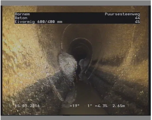
Corrosion, surface erosion and encrustations are flaws that occur on the inside of the pipe. As Kaempfer and Berndt (1999) mentions, the severity of corrosion depends on the surface pH value. Surface erosion and encrustations depend on the amount of water that flows through the pipe, but also what kind of stuff is dumped into the sewers (Kaempfer and Berndt, 1999). Figure 2.64shows the visible effect of corrosion on the sewer pipe. Figure 2.75illustrates the effect of encrustation in the pipe.

Figure 2.6:Corrosion on inner surface of pipe Figure 2.7:Encrustation inside the sewer pipe

2.1.6 Tree roots

Tree roots also play a small role in the distribution of flaws in sewer pipes. Roots of trees occa-sionally grow into the pipe through cracks and joint displacements (Randrup et al., 2001). In figure 2.86an example of the flaw is given.

3_{https://hoodline.com/2016/05/what-you-should-know-about-sinkholes} 4_{http://www.maverickinspection.com/services/remote-video-inspection/}

rvi-video-imagery-gallery/drainage-systems/

5_{http://blog.envirosight.com/the-cost-of-sewer-pipe-corrosion}

Figure 2.8:Root growth inside sewer pipe

As the figure shows, tree roots are clearly visible on camera during in-pipe inspection.

2.1.7 Conclusion

2.2 Relation between material properties and structural flaws

In the previous section the flaws that need to be located with physical interaction inspection is discussed. This section will discuss the relation between measurable physical properties and voids and cracks. Therefore this section will answer the following sub-question:How do mea-surable physical properties of the concrete pipe relate to these structural flaws?.

In order to relate measurable physical properties to structural flaws, two measurable physi-cal properties of concrete will be mentioned and explained:the elastic modulus and the com-pressive strength. At the end of this section a conclusion will be made of how the measurable physical parameters are influenced by the structural flaws.

2.2.1 Elastic modulus

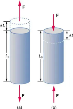
The elastic modulus of a material is based on the relation between the stress and strain of the material. In order to determine the elastic modulus of a material, a force is applied on a cylinder of this material. This can be in the compression direction or in the tension direction. Figure 2.9

7_{will be used to explain how the elastic modulus of a material is determined.}

Figure 2.9:Deflection of a cylinder

The strain is determined by the difference in length,∆L, divided by the original lengthL0. The

stress is determined by the force,Fdivided by the area of the cylinder, A. When the stress on such a cylinder is plotted against the strain, it is called the stress strain curve. This stress-strain curve is shown in figure 2.108.

7_{https://opentextbc.ca/physicstestbook2/chapter/elasticity-stress-and-strain} 8_{https://www.pavementinteractive.org/reference-desk/design/design-parameters/}

Figure 2.10:Stress strain relation

The elastic modulus is the relation between stress and strain in the elastic range of the stress strain curve. This relation is actually the slope of the curve, visible in figure 2.10. The elastic modulus of concrete is about 30 GPa9, but can be different for different kind of concretes, as it depends on how the concrete is made (Counto, 1964) (Hirsch, 1962). For comparison, the elastic modulus for rubber is between 0.001 GPa and 0.05 GPa10.

2.2.2 Compressive strength

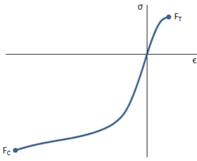
The compressive stress under which the material breaks, is called the compressive strength. This is in the opposite direction with regard to the tensile strength, which is the tensile stress under which the material breaks. In figure 2.1111the stress-strain curve of brittle materials is shown, from which the tensile strength and the compressive strength can be interpreted.

Figure 2.11:Stress strain relation for brittle materials

In the stress strain curve, the compressive strength is the stress on the lowest point of the curve,

FC. The tensile strength is the highest point on the curve, FT. For metals the compressive

strength and the tensile strength are similar (Tort et al., 2010). Concrete however, is stronger in compression than tension, which is also shown in figure 2.11. A rule of thumb is to assume that

9_{https://www.engineeringtoolbox.com/young-modulus-d_417.html} 10_{https://www.azom.com/properties.aspx?ArticleID=920}

the compressive strength of concrete is ten times stronger than the tensile strength of concrete (Badarloo et al., 2018), where the compressive strength is on average 40 MPa12. In case of rubbers it is the other way around, the tensile strength is higher than the compressive strength (Al-Mosawi, 2015), the compressive strength of rubber is on average 7 MPa (Fediuc et al., 2013). Figure 2.10 is actually quite similar to figure 2.11, where the first figure did only show the tensile range.

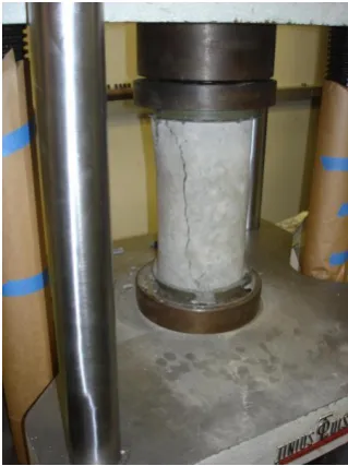
The most reliable way to determine the compressive strength of concrete is to increase the applied force until it actually breaks. While this gives the most reliable value for the strength of the material, the tested material is afterwards destructed. This is the so called ’Destructive test’. For this test, a concrete cube or cylinder is crushed in a compressive strength test by pressing on the sample and increase the stress until it breaks. An example of the compressive strength test is shown in figure 2.1213.

Figure 2.12:Example of compressive strength test on concrete

The figure shows an example of the destructive test. As mentioned, the test destroys the sample, which makes it unsuited for testing concrete structures which are in use, like sewer pipes. There also exist quite some non-destructive methods which estimate the strength of the concrete structure. An example is the Schmidt hammer, which will be discussed in section 2.3.

2.2.3 Relation between measurable material properties and cracks in concrete

In order to determine if the measurable material properties are affected by cracks, research based on literature is conducted. Cracks appears to be related to the compressive strength of concrete (Vecchio and Collins, 1993), as cracks soften the material and consequently lower the compressive strength. Vonk (1992) states the following: ’Analysis of test results shows that the size effect in compressive softening is more complex than in tensile softening. Localization of cracking is present in compressive softening, but it has a more diffuse character than in tensile softening.’ Micro cracks also reduce the elastic modulus, due to softening (Maruyama et al., 2014). Dyskin et al. (2003) studied the crack propagation in cement under uniaxial loading of initial 3D cracks, where the existence of initial cracks influenced the maximal loading capacity. The size and orientation of the crack have also influence on this maximal loading capacity. A reduction of the compressive strength due to cracks is to be expected in concrete, however

12_{https://www.engineeringtoolbox.com/young-modulus-d_417.html}

according to Vonk (1992) this relation has a diffuse character, so it is not certain that this flaw will be measured. As time is limited, this research will not focus on the microscopic influence of cracks on the material behavior. Additional research is however required on how cracks influence the strength of the material, especially how they influence the compressive strength and elastic modulus of the material.

2.2.4 Relation between measurable material properties and voids in concrete

Research is also conducted on the relation between the measurable material properties and voids in concrete. Comparable to cracks, voids also reduce the compressive strength of the con-crete (Ezeokonwo, 2000). Ezeokonwo (2000) tested different strengths of concon-crete with voids with different sizes and different orientations. Figure 2.13 shows the relation between the size and orientation of a void on concrete.

Figure 2.13:Influence of size and orientation of void on compressive strength (Ezeokonwo, 2000)

The figure clearly shows a decrease of compressive strength of the concrete due to the presence of a void. As well as the size as the orientation of the void influence the compressive strength. On the contrary, small air voids in concrete do actually increase strength of the concrete (War-ren, 1953).

To gain insight on the influence of a void in a concrete tile on the strength of the tile, a finite element study has been conducted. A simulation has been done in order to calculate the de-flection caused by a load on the tile. This is also done for a tile with a void. Both dede-flections can be compared in order investigate the influence of a void. These simulations where conducted in COMSOL Multiphysics. The used variables are shown in table 2.1 and the result is shown in figure 2.14.

Table 2.1:Displacement estimation with Elastic modulus

Variable Value Unit

Force 50 N

Elastic modulus 30 GPa

Figure 2.14:Modelled deflection of tile in COMSOL Figure 2.15:Modelled deflection of damaged tile

The largest displacement is in the middle of the undamaged tile, at the point of pressing, and is 0.0231µm. In figure 2.15 the simulation is shown in the case of a damaged tile, where the largest displacement is 0.962µm. The displacement on the tile with a void is about forty times larger than the tile without any damage. This simulation indicates a decrease in strength for a big void, however, no literature could be found on that subject. There needs to be noticed that in both cases the displacement is very small.

2.2.5 Conclusion

2.3 Rebound principle of assessing concrete

In the previous section the relations between the elastic modulus and the compressive strength and potential flaws are shown. In this section will be discussed how the rebound hammer is able to determine the compressive strength of concrete and the hammer will be compared with the Leeb hammer, which uses an impact to determine the hardness of the material. The working principle of the Leeb hammer and the Schimdt hammer will be investigated. In this section an answer will be given on the following question: What principle do the Schmidt hammer and Leeb hammer use to asses the concrete?

Firstly, an explanation will be given on how the rebound hammer works and how to operate the hammer. Next its principle will be explained. Secondly, the working principle of the Leeb hammer will be explained. The leeb hammer and the rebound hammer will be compared and it will be discussed what the hammers actually measure. Accordingly an answer will be given on the sub-question.

2.3.1 Rebound hammer

The rebound hammer is used in the civil engineering to determine the compressive strength on-site. In this section is explained how the hammer works and its required conditions are mentioned. Then the principle of the hammer will explored more deeply in order to determine what the hammer actually measures.

In order to explain how the rebound hammer works, different states of the hammer are shown in figure 2.16.

Figure 2.16:Different stages rebound hammer (Kvgd and Yelisetty, 2014)

means the hammer did not bounce back and a value of one hundred means the hammer did bounce the whole distance back. Based on these distances the rebound value is determined and shown on the indicator. This rebound value is a relative indication of the strength of the material, where the rebound value can be used for comparison of the strength between two samples under similar conditions. In practice it is desired to relate the rebound value to the compressive strength of the sample. In order to do so, the hammer needs to be calibrated on a calibration anvil. After calibration the rebound value can be used to determine the compressive strength using a conversion. Figure 2.17 shows a conversion figure to estimate the compressive strength of the sample based on the measured rebound value, for the N/NR Schmidt hammer (EngineersDaily, 2019). Figure 2.18 shows the conversion graph for a L/LR Schmidt hammer.

Figure 2.17: Conversion graph for N/NR Schmidt hammer (EngineersDaily, 2019)

Figure 2.18: Conversion graph for L/LR Schmidt hammer (EngineersDaily, 2019)

The conversion curve shown in the figure, only holds for tests on a concrete cube, with sides of 150mm. The sample should have a smooth, dry surface, without any flaws in the cube. The concrete also should have an age between 14 and 56 days. The maximal diameter of the aggre-gate has to be 32 mm. In case the conditions differ from the required conditions for the con-version table, a factor is required in order to relate to the compressive strength. In the manual and literature certain formula are described which can be used to apply a factor to the mea-sured rebound value to determine the rebound value of the material. The required conditions are quite a limitation on the technique, as unknown deviations give an error in the estimation of the compressive strength. Another limitation is the accuracy of the rebound method, as the method is very inaccurate. To get a good indication of the strength of the material and reduce the effect of the inaccuracies, it is advised to do a minimum of ten measurements and take the average value (ReboundGuide, 1993). The graph in figure 2.17 shows three lines, each with a position of the hammer drawn. This illustrates the effect of the orientation on the conversion between the rebound value and the compressive strength. This conversion is required as the gravity influences the measured rebound value. Figure 2.17 also mentions that the conversion table is to be used for the N/NR hammer. This N-type hammer is a hammer that uses an im-pact energy of 2.2 J and is supposed to be used on concrete with a thickness between 50 mm and 100 mm. Another rebound hammer is the L/LR hammer, which is an hammer that uses an impact energy of 0.72 J (ReboundGuide, 1993). What can be seen in the conversion graphs in figure 2.17 and figure 2.18 is that the LR hammer has a higher rebound hammer for sam-ples with the same strength. This gives an indication, that a higher impact energy results in measuring a higher rebound value.

de-termine the rebound value, where the rebound value depends on the initial position and the position to which the hammer bounces back.

R=xr x0

(·100) (2.1)

WhereR is the rebound value. The rebound value is multiplied by 100 so it actually shows a percentage, in future equations the value without the multiplication of 100 is used. xr is the

measured rebound distance andx0 is the start position of the hammer. The impact energy

originates from the initial stored energy in the system, which is the spring energy. The formula for this energy is shown in equation 2.2.

Ek,0=

1 2C x

2

0 (2.2)

WhereEk,0 is the initial energy, which is the spring energy. C is the spring constant of the

rebound hammer. When assuming the influence of friction and gravity can be neglected, where the influence of gravity can be neglected in the case of applying a horizontal impact, all this energy converts into kinetic energy. On the moment of impact this kinetic energy will cause the material to deform partially elastic and partially plastic. When the energy lost to heat and the creation of sound is neglected, all the energy is converted into either strain energy or energy stored into plastic deformation.

The strain energy will convert into kinetic energy of the hammer at the end of the impact, when it will move the hammer back up. The energy stored into plastic deformation will be lost. The maximal strain energy can be estimated by equation 2.3.

Estrain=

1 2C x

2

r=

1 2C·x

2 0

x2_r

x2₀ =E0·R

2 _(2.3)

WhereRis the rebound value, shown in equation 2.1.E0is the initial energy, shown in equation

2.2. The energy lost due to the plastic deformation can therefore be approximated by equation 2.4, because it is assumed that the energy lost to plastic deformation is the initial energy minus the strain energy.

Eplastic=E0−Estrain=E0(1−R2) (2.4)

These equations mainly show that the rebound value measures the plastic deformation caused by the impact. As Szilágyi et al. (2015) states "The value of the coefficient of restitution depends on energy losses due to dissipation by reflections and attenuation of mechanical waves inside the steel plunger and energy losses due to dissipation by concrete crushing under the tip of the plunger. This latter loss of energy makes the rebound hammer suitable for strength estimation of concrete. The energy dissipated in the concrete during local crushing initiated by the impact depends both on concrete compressive strength and Young’s modulus; therefore, depends on the stress-strain (σ−²) response of the concrete tested."

related to the gravity. The output velocity divided by the input velocity is called the true re-bound coefficient, as shown in the following equation.

Q=vout vin

(2.5)

WhereQis the true rebound coefficient,vout is the velocity after the impact andvinis the

ve-locity before the impact. According to the research of Winkler and Matthews (2014) the Silver Schmidt Hammer realizes comparable results. This makes a lot of sense when looking at the initial energy and rebound energy again. Instead of looking at the initial spring energy, a look will be given to the initial kinetic energy.

Ekin,0=

1 2mv

2

in (2.6)

The energy after the impact can be based on the kinetic energy based on the velocity after the impact.

Erebound=

1 2mv

2

out (2.7)

Rewriting this equation will give the following equation.

Erebound=

1 2mv

2 in·

v_out2 v2_in =E0·

v2_out

v_in2 (2.8)

This shows the same structure as 2.3, where the first part is equal to 2.6 and the second part to the rebound value. This gives the following equation for the rebound value.

Q=vout vin ≈

R=xout xin

(2.9)

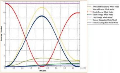
Contrary to the rebound value,Q is not influenced by the gravity so conversion based on the direction of the gravity is not required. As this equation shows that the different type of measur-ing should give similar results. It is important to remember the made assumptions; The effects of friction and viscous energy dissipation are disregarded. In reality these effects will influence the measurements. The influence of these effects are shown in figure 2.19. This figure shows the model of the energy balance during an impact (Patel et al., 2014). This study uses a model with a low-velocity impact, where the velocity of impact is considered 1 m s−1to 3 m s−1, using ABAQUS Explicit. In figure2.19 the impactor mass is 2.6 kg, the velocity 3 m s−1and the longi-tudinal compressive strength of the sample is considered 350 MPa (Aslan et al., 2003), which is higher than the compressive strength of concrete.

As the figure shows, the kinetic energy, in this case 12 J, is mainly converted into strain energy, which then converts back into kinetic energy. Energy is also lost to frictional dissipation, vis-cous dissipation and artificial strain energy. The final artificial strain energy can be considered as the plastic deformation. The figure shows that while the frictional dissipation and the vis-cous dissipation is small, it influences the energy lost during an impact.

2.3.2 Leeb hammer

Figure 2.19:Impact model of Patel et al. (2014)

Figure 2.20:Description of working principle of Leeb hammer (Kovler et al., 2018a)

The loaded spring will cause the impact body to move with a certain velocity. The impact will cause the impact body to rebound. The relation between the rebound velocity and the input velocity is used to determine the hardness of the body tested. The Leeb hardness is determined on these velocities according to the following equation.

H L=vout vin ·

1000 (2.10)

Wherevoutis the rebound velocity,vinthe impact velocity andH Lthe Leeb hardness. The Leeb

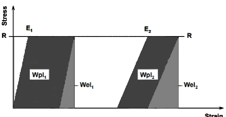
Figure 2.21:Influence of elastic modulus on rebound hammer (Kompatscher, 2004)

This figure is a simplified representation of the stress-strain curves of two materials with the same compressive strength, but different elastic moduli. In the figureRstands for the Yield strength, which is equal for both materials shown in the graph. E1andE2stand for the

elas-tic modulus of the two materials. The relation between Wel1and Wpl1yields a significantly

higher value than the relation between Wel2and Wpl2 while the yield strength is equal. This

illustrates that a material with a lower elastic modulus will yield a higher rebound value, while the compressive strengths are equal.

2.3.3 Comparison of Rebound hammer and Leeb hammer

In this section the rebound hammer and the leeb hammer will be compared. Both hammers use the rebound principle. However, the leeb hammer uses a much lower impact energy. On top of that, contrary to the regular Schmidt hammer, the rebound value of the leeb hammer and the Silver Schmidt hammer are not influenced by the direction of the test with regard to the direction of gravity. The figures 2.22 and 2.23 show the relation between their rebound number and the compressive strength (Kovler et al., 2018b).

Figure 2.22: Relation between rebound value and compressive strength.

The figures show that the Leeb hammer is in the study of (Kovler et al., 2018b), quite more accu-rate in determining the compressive strength of a material than the regular rebound hammer, as the confidence band is much smaller. On the contrary, Szilágyi et al. (2015) claims that the Leeb hammer rebound value is actually more related to the elastic modulus of the material than the compressive strength, due to the low impact energy. Szilágyi et al. (2015) supports the latter claim by figure 2.24 (Szilágyi et al., 2015).

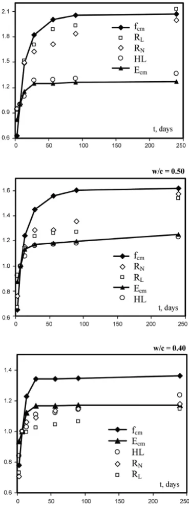
Figure 2.24:Relative change of modulus, strength and rebound values over aging of concrete.

Wherefcmis the compressive strength of the concrete sample over time andEcm is the elastic

In the study, three different mixtures of concrete are tested, where the w/c ratio is the ratio be-tween the water and the cement. The mixture of 0.4 w/c has a significantly higher compressive strength and elastic modulus than the mixtures with a higher w/c ratio. What can be seen in the figure is that the strength over time increases as the concrete dries. The figures shows that the Leeb hammer values correlate with the elastic modulus. The rebound hammer correlates with the compressive strength for mixtures with a higher w/c, but also correlates with the elastic modulus for the concrete with a 0.4 w/c ratio. Szilágyi et al. (2015) concluded the following: "Results demonstrated that the rebound hammers could provide a hardness value that can be correlated to the compressive strength of concrete only if the compressive strength is relatively low. It was confirmed for high strength concretes that the Schmidt rebound hammers provide a hardness value that can be correlated to the Young’s modulus of concrete rather than the compressive strength."

However, the study uses the development of the elastic modulus and the compressive strength of concrete over time. The study therefore neglects other effects that happen over time with the concrete that can influence the measured rebound values with the different hammers.

Kovler et al. (2018a) also compared the values given by the Schmidt hammer and the Leeb ham-mer. This comparison is shown in figure 2.25.

Figure 2.25:Comparison between Schmidt hammer and Leeb hammer (Kovler et al., 2018b)

In the figure values on relatively young concrete are shown and values on old concrete are shown. Kovler et al. (2018a) expects that the difference in relation between the hammers can be explained due to the fact that the Leeb hammer measures on the surface, where this surface is greatly influenced by aging due to carbonation. The Schmidt hammer is less influenced by this effect, as it measures the strength of the material and therefore less on the surface.

2.3.4 Conclusion

2.4 Robotic assessment of concrete based on the rebound principle

In the previous section is explained how the rebound principle is used to asses the strength of concrete. This section will explain how this principle can be used by assessing concrete with a robotic arm, this in order to answer the following sub-question:How can the rebound hammer principle be used to locate structural flaws with a robotic arm?

In order to answer this question specifications of the robotic arm are given. Then there will be explained how to mimic the principle of the hammers with a virtual spring. How to implement a virtual spring by using impedance control will be explained. Accordingly how to estimate the external force applied on the end-effector will be explained.

2.4.1 Impact test with virtual spring

In order to mimic the principle of the rebound hammer, the energy loss to plastic deformation should be determined. A virtual spring will be placed at the end-effector, as shown in figure 2.26, which imitates the effect of the spring of the Silver Schmidt hammer. The mass of the robotic arm imitates the effect of the mass attached to the spring of the hammer.

Figure 2.26:Overview of virtual spring attached to the end-effector of the robotic arm

The virtual spring instantly attached to the end-effector will cause the end-effector to be drawn towards the surface of the sample and impact the surface with a certain impact energy. Accord-ingly, the hammer will bounce back on the surface with a certain speed. Based on the velocity at impact and the velocity when bouncing the rebound value should be determined. This velocity response of the Leeb hammer is shown in figure 2.27 (Kovler et al., 2018a).

A similar velocity response is expected when impacting with a robotic hammer and the re-bound value will be determined based on the rere-bound velocity relative to the initial velocity. This rebound value relates to the compressive strength, which then again is related to cracks and voids in the concrete. Therefore it is expected that impacting a surface with a robotic arm can be used to determine a certain rebound value that is related to the relation between the elastic modulus and the compressive strength.

R=vout vin

(2.11)

Wherevoutis the maximal velocity of the end-effector after the impact andvinis the velocity

of the end-effector at impact. This is the same relation as used by the Leeb hammer, similar to the Leeb hammer, it is therefore assumed that the direction of impact with respect to the direction of the gravity has no considerable influence on the measured rebound value. Based on the analysis in section 2.2 the rebound value is expected to be lower in the case of flaws. Therefore it is expected that the impact with a robotic arm can be used to locate flaws based on the rebound value, where the rebound value can be used as relative measurements. An experimental study is however needed in order to determine whether this is actually the case.

In order to determine the rebound value, the velocity of the end-effector should be determined. This velocity can be determined based on the angular velocity of the joints. The relation be-tween these velocities is shown in equation 2.12.

T₀n=J(q)·θ˙n (2.12)

WhereT₀n is the twist of the end-effector with respect to the base frame, where the velocity in the Cartesian frame can be determined based on the twist. ˙θn is a vector containing the

mea-sured angular velocities in the joints.J(q) is the Jacobian, which depends on the configuration. The Jacobian will be explained in the next subsection.

As shown in section 2.3.2, the Leeb hardness not only depends on the yield strength, but also on the elastic modulus. Because this method will use the same impact principle, it is expected that a similar relation between the elastic modulus and the compressive strength will be mea-sured. This could be tested by impacting on a material with a much lower elastic modulus, but a similar compressive strength, as a higher rebound value is expected for that case.

2.4.2 Jacobian

In order to determine the velocity of the end-effector in equation 2.12, the Jacobian has to be determined for each configuration. The Jacobian for a seven degrees of freedom serial robotic arm can be given by the following equation (Stramigioli and Bruyninckx, 2001).

J=£Te1 Te2 . . . Ten ¤

(2.13)

Where J is the Jacobian andTei is the twist of each joint. In this case the Jacobian does not

2.4.3 Impedance controller

The virtual spring attached on the end-effector can be realized by using an impedance con-troller. A controller in the Cartesian frame can be simplified into the following equation.

~

Fvirtualspring= −K~e−D~x˙ (2.14)

Where~Fvirtualspringis the force of the virtual spring-damper acting on the end-effector.Kis the

stiffness matrix,D is the damping matrix. ~eis the error between the desired position of the spring and the position of the end-effector.~x˙is the velocity of the end-effector in the Cartesian frame. Based on the task force the task torques for the joints can be determined using the transpose of the Jacobian.

~τvirtualspring=J(q)T~Fvirtualspring (2.15)

WhereJ(q) needs to be transposed and~Fvirtualspringis calculated in equation 2.14.~τvirtualspring

is a vector containing the torques in each joint that represent the force applied by the virtual spring on the end-effector.

The stiffness matrix is determined based on the following equation.

K=

·_K

translation 0

0 Krotation ¸

(2.16)

Where the translation stiffness matrix and rotation stiffness matrix are three by three matrices. For simplified usage only the diagonals will be used. The stiffness matrix for translation can be formed by the following equation.

Ktranslation=I3~kt r ansl at i on (2.17)

Where~kt r ansl at i onis a vector of three elements, where each element represents a stiffness of a

direction in the Cartesian frame.I3is an identity matrix (3x3).

~kt r ansl at i on=

  kx ky kz   (2.18)

Krotationis configured the same way asKtranslation, but then depends on the desired stiffness for

rotation. As the equations are similar, this will not be explained in the same detail asKtranslation.

The damping matrix,D, from equation 2.14, is configured the same way as the stiffness ma-trix,K, but different values can be used in order to add damping to the system. A generally used value for damping is 2pkfor each direction, wherekare the stiffness values used for the stiffness matrix.

The virtual spring energy depends on the configured spring distance and the spring coefficient, as the spring energy is given by the following equation.

Espring=

1 2C x

2 _(2.19)

damage on the robot itself. The actual impact energy that can be achieved with the robotic arm, can be determined based on the kinetic energy. The kinetic energy can be determined based on the mass of the links of the robot and the velocity of the joints, as shown in the following equation.

Ekin=

1 2~q˙

T_M(q)~_{q˙ (2.20)}

Where~q˙is a vector of the velocities of the joints andM(q) is the mass-matrix of the robot, which depends on its configuration. The impact that should be applied in order to locate structural flaws will be discussed in the experimental study in the next chapter.

In theory the spring distance and spring stiffness will only influence the impact energy. The spring distance and stiffness itself are not expected to influence the results. This should be tested by applying the same impact energies but with different distances and stiffness settings. Also the influence of damping should be revised. Damping is desired, as otherwise stability issues are to be expected, however added damping could influence the results. The robotic arm itself has also damping, due to friction. Looking at the influence of damping will also give an idea of the influence of the friction of the robotic arm. In case the influence is severe, compensation for friction can be considered as a solution.

2.4.4 Aspects to take into account when measuring with a robotic arm

As mentioned in section 2.4.2, inaccuracies on the measurements are expected due to deflec-tions in the arm, while the stiffness of the arm will depend on its configuration. The stiffness of the arm is unknown and needs to be determined, accordingly the influence of the configura-tion on the rebound value needs to be determined via experimental data. The influence on the measured position and velocity of the end-effector is important, as the relation between the impact velocity and the rebound velocity are used to asses the concrete.

2.4.5 Conclusion

In this section is discussed how to locate structural flaws in concrete sewer pipes with a robotic arm by using a virtual spring in order to use the rebound hammer principle of the leeb hammer and the Silver Schmidt hammer, where the impact velocity can be related to the rebound veloc-ity. This virtual spring can be made by using impedance control. In this section the equations for the impedance controller were shown and several variables were mentioned. The impact energy is expected to be of influence on the rebound value, as the impact energy seems to play a role of importance for differences between the Schmidt hammer and the Leeb hammer, as discussed in section 2.3.3. The maximal impact energy that can be applied on assessing con-crete is however unknown, during the experimental study the maximal impact energy will be discussed. Furthermore it is important to investigate the accuracy of the velocity measurement of the end-effector, as this is used to determine the rebound value. In order to validate the as-sessment method test needs to be performed on a material with a different relation between elastic modulus and compressive strength, a concrete tile with a void and a concrete tile with a crack.

2.5 Conclusion of analysis

3 Experimental Study

In the previous chapter the feasibility of locating structural flaws is analyzed. As mentioned, experimental study is required in order to determine if the rebound value of a sample can be determined properly with a robotic arm. In this chapter the proposed method to locate struc-tural flaws will be tested, in order to answer the question: ’To what extend can interaction between a robotic arm and the surface of a concrete pipe be used to locate structural flaws of the pipe?’

First the design of the experimental setup will be explained. Secondly the different experiments that will be conducted will be mentioned. Then each experiment will be discussed separately, by explaining the experiment, showing its results and discussing the results. At the end of this chapter the overall results of the experimental study will be discussed.

3.1 Design of experimental setup

In this section the design of the experimental setup will be discussed. First an overview of the setup will be shown. Then the separate parts of the experimental setup will be mentioned and their specifications will be given.

3.1.1 Overview

In this section an overview of the experimental setup is given. A schematic overview of the experimental setup is shown in figure 3.1.

Figure 3.1:Schematic overview of experimental setup

Figure 3.2:Picture of experimental setup

The picture shows the robotic arm with respect to the sample and the video camera. The cam-era is placed with a distance of 50 cm to the end-effector. One can also see the force sensor at the end-effector.

3.1.2 Robotic arm

For the experiments the ’Panda’, manufactured by Franka Emika, will be used for the experi-ments. A picture of this robotic arm is shown in figure 3.31.

Figure 3.3:The Panda, manufactured by Franka Emika

The specifications of the panda are given in table 3.1. Additional specifications of the robot, like the dh-diagram and the contact limitations of all joints, can be found in appendix A.

Table 3.1:Panda specifications

Specifications Value Unit

Repeatibility error 0.1 mm Cartesian velocity limit 1.7 m s−1 Cartesian acceleration limit 13 m s−2 Degrees of freedom 7

Communication rate 1 kHz Maximum contact force 140 N

Payload 3 kg

As the table shows, the maximal contact force is 140 N. This is one of the limitations with regard to the maximal impact energy. Also the Cartesian velcoity limit and the Cartesian acceleration limit should not be exceeded upon impact. Furthermore, the joint limitations shown in ap-pendix A should also not be exceeded.

1_{http://donar.messe.de/exhibitor/hannovermesse/2017/X376456/}

In order to control the robotic arm, a interface has to be used: The Franka Control Interface (FCI). A schematic overview of the communication between a workstation PC and the FCI is shown in figure 3.42.

Figure 3.4:Schematic overview of Franka Control Interface

As the figure shows, communication can be achieved at a communication rate of 1 kHz. Com-mands have to be sent to the FCI and measurement data will be provided to the workstation PC. This measurement data includes measured torques in the joints and the angular position of the joints. The FCI does however also include a library which enables to receive the Jacobian at a certain configuration, the inertia matrix, the Coriolis and centrifugal vector and the gravity compensation torques. It also enables the external force estimation based on the measured torques, minus the Coriolis, centrifugal and gravity compensation, with a filter included. In-stead of implementing functionality in order to estimate these values, the FCI library will be used to do so. The libfranka library is used to control the robotic arm. The available impedance controller is implemented by including the control into a cpp file. There has been chosen to use an impedance controller as this controller represents a virtual spring, which is used to mimic the spring used in all the rebound hammers.

3.1.3 Force sensor

In section 3.1.1 the use of a force-torque sensor is mentioned. This sensor is connected with screws on 3D-printed material, which is then connected to the robotic arm. The force sensor is used in order to validate the estimation of the external force applied on the end-effector. The force-torque sensor used is the Schunk mini-40-SI-80-4. In figure 3.53a picture of the force sensor is shown.

Figure 3.5:Schunk mini-40-SI-80-4

2_{https://frankaemika.github.io/docs/overview.html}

3_{http://sciencedocbox.com/Physics/75355109-Product-information-force-torque-sensor-ft.}

The ROS package netft_utils is used to extract the data from the force sensor. The measure-ments will be biased into zero when attached to the robotic arm in order not to measure the gravity force applied on the material attached to the force sensor.

The external force applied on the end-effector can also be determined based on how the ex-ternal force affects the torques of the joints. The exex-ternal force acting on the end-effector can be determined by multiplying the inverse of the Jacobian with the external influence on the torques of the joints. In the case the Jacobian is not invertible, the pseudo-inverse of the Jaco-bian with the external influence on the torques of the joints should be used to determine the external force, which is shown in the following equation.

Fext=J†·τext (3.1)

WhereFextis the external force on the end-effector andJ† is the pseudoinverse of the Jacobian.

τextis the external effect on the torques of the joints, which can be determined by the measured

torque minus the effect of gravity, Coriolis and friction, as shown in the next equation.

τext=τmeasured−τg−τCoriolis−τfriction (3.2)

τmeasuredis the measured torque,τg the torque in order to compensate gravity andτCoriolisis

the influence of the Coriolis effect on the torque. This research will not go into depth how to determine these torques. Ott et al. (2004) shows how to determine the torque needed for gravity compensation,τg. Pigeon et al. (2013) shows how to determine the torque to compensate the

Coriolis effect. With the values for these torques,τext, the effect of the external force on the

torques, can be determined. This can be used in order to determine the external force as shown in equation 3.1.

3.1.4 High speed camera

As mentioned in section 3.1.1 a high speed camera is used to validate the movement estimation of the end-effector. In this section the specifications of the high speed camera and the software used for image processing will be mentioned. The camera itself is shown in figure 3.64.

Figure 3.6:Camera used for high speed filming, Nikon 1 j4

The shown camera is the Nikon 1 j4 and is placed 50 cm away from the point of impact. The camera can film in HD quality (1920x1080px) at 29.97 frames per second. The camera also has a slow motion feature, where it can film at 400 frames per second or 1200 frames per second for three seconds, the quality is decreased by a higher frame rate. 416x144px for 1200fps and 768x288 for 400fps. In figure 3.7 a frame of a video at a frame rate of 400 frames per second is shown and in figure 3.8 a frame of a video at a frame of 1200 frames per second is shown.

Figure 3.7:One frame from video of 400fps Figure 3.8:One frame from video of 1200fps

Both images show a clear difference in clarity of the image. The frame of the 1200 fps video shows the influence of the smaller resolution. The video of 400fps is therefore expected to measure the distance traveled by a point between two frames to be more precise. However also more time is passed between two frames with respect to the video of 1200 frames per second. Because of the resolution the impact will be captured with 400 frames per second. The captured video will be discussed and then it will be determined if 400 frames per second are enough to measure the impact velocity and the rebound velocity.

In order to determine the velocity of the end-effector based on the video, image processing is required. Kinovea image processing tool will be used in order to do so. The yellow dot on the blue printed plastic, visible in figure 3.7, for which the position will be determined. In order to relate the position in pixels to distance in meters, the length of the blue printed material will be used, which is 2.3 cm. In order to determine the velocity based on the position change over the frames, Kinovea has filtering included. The program uses two passes of a second order Buttersworth filter; One foward and one backward, in order to reset the phase shift (Winter, 2009). Every point is extrapolated 10 points on each side in order to initialize the filter (Smith, 1989). The cutoff frequency is determined based on the estimation of the autocorrelation of residuals, by finding the frequency that yields the residuals that are the least autocorrelated. The filtered data set corresponding to this cutoff frequency is kept as the final result (Challis, 1999). The Durbin-Watson statistic is used to estimate the autocorrelation of the residuals. This filtering is a built-in feature of Kinovea and will be used as intended.

3.1.5 Virtual spring

Impedance control will be used to place a virtual spring between the sample and the end-effector. In this section the implementation of the impedance control will be described. Also the variables which will be used for the experiments are mentioned.

The impedance controller, mentioned in the analysis in section 2.4.3, is implemented in order to do an impact test. For the implementation has been chosen to further simplify the virtual spring in order to reduce the parameters for the tests. The impact will be applied in one direc-tion only. A schematic representadirec-tion of the virtual spring is shown in figure 3.9.

Figure 3.9:Schematic representation virtual spring

as variablelk. To test the feasibility of the method, there has been chosen to only test in the

z-direction. The distances described in the figure are therefore one-dimensional. The distance between the surface and the starting point does not necessarily have to be equal to the length of the spring, as figure 3.9 shows. The relation between these distances can be described by the following equation.

rd= lk ds

(3.3)

Wherelkis the length of the spring,dsis the distance between the starting point and the surface

andris the dimensionless value with represent the ratio between the two lengths. The variables which can be used to set the spring areds andr.

Figure 3.9 also shows the valuek, which represents the stiffness of the spring. Equation 2.17 and 2.18 showed that a simplified impedance Cartesian impedance controller can be set with three stiffness properties, one for each direction.

~kt r ansl at i on=

  kx ky kz   (3.4)

As the spring is simplified to be one directional, the stiffness that will influence the impact energy iskz. The other stiffness properties,kxandky are set very high, namely 5000 N m−1, so

the impactor will be guided into being applied in one direction, which can be compared with the housing of a rebound hammer.kzis a variable of the impedance controller that should be

tuned for the experiments.

In section 2.4.3 is mentioned how the virtual spring energy can be determined. Because the vir-tual spring is simplified to the one dimensional case, the spring energy depends on the length of the spring and the spring stiffness. However, when the spring is placed under the surface of the sample, not all the spring energy will be converted into kinetic energy. The following equation represents the effective spring energy.

Espring,eff=

1 2kzl

2

k−

1

2kz(lk−ds)

2 _(3.5)

The impact energy is however the spring energy that is converted into the kinetic energy. The spring energy can also be lost due to friction before the impact is achieved. The kinetic en-ergy at impact will be considered as the impact enen-ergy and can be determined based on the following equation, as mentioned in section 2.4.3.

Ekin,in=

1 2~q˙

T

i nM(q)~q˙i n (3.6)

Where~q˙i nis the angular velocity of the joints at impact andM(q) is the mass matrix.

3.1.6 Samples

Figure 3.10:Concrete tile Figure 3.11:Concrete tile with a crack

On one tile, with the thickness of 4.5 cm, a crack has been induced, figure 3.11. Another tile, with the thickness of 8.5 cm has been damaged by making a void on the back of the tile, figure 3.13.

Figure 3.12:Two concrete tiles, 4.5 cm and 8.5 cm Figure 3.13:Concrete tile with a void

Figure 3.14:Upside of rubber tile Figure 3.15:Downside of rubber tile

These samples will be placed on a table in order to induce an impact test on the sample. In figure 3.16 the placement of a sample on the table is shown, where the middle of the sample will be placed at a distance of 60 cm in y direction from the robotic arm.

Figure 3.16:Placement of sample with axis

3.1.7 Impact Test

Figure 3.17:Activity diagram of impact test

The figure shows the various steps of the impact test. The rebound value for each impact test will be determined based on the rebound velocity divided by the impact velocity, as discussed in section 2.4. During the velocity response will be used in order to determine the rebound value. A velocity response that could be expected is shown in figure 3.18.

Figure 3.18:Expected velocity response of impact

3.2 Description of experiments

As concluded in the analysis, a variety of tests is required in order to determine if a robotic arm is able to locate structural flaws in concrete. In this section will be discussed which experiments will be conducted, based on the analysis.

3.2.1 Validation impact test

The design of the experimental setup explains how the robotic arm will be used to determine the rebound value. The goal of the first experiment is to validate the impact test. This will be achieved by determining the velocity of the end-effector based on the angular velocity of the joints and compare this velocity with the velocity measured with the high-speed camera. Then the rebound value will be determined for multiple tests on the same position in order to determine the variance of the rebound value test with a robotic arm. This rebound value and variance will be compared with a rebound value test with a Schmidt hammer on the same position as the robotic arm tested the rebound value.

3.2.2 Internal deflection robotic arm

As mentioned in the analysis, in section 2.4.1, deflection of the arm can influence the measured velocity. To analyze the performance of the impact test, it is therefore necessary to determine the influence of the stiffness of the arm on the measured value. Tests are required in order to determine the stiffness of the robotic arm. This is also required in order to relate this research to the use of other robotic arms.

When the stiffness properties of the robotic arm are determined, the influence of these stiffness properties on determining the velocity and the rebound value should be investigated. This can be achieved by comparing the velocity of the end-effector based on the measurements of the angular velocity of the joints with the velocity of the end-effector determined by the image processing of the video captured by the high speed camera for the different positions. A look will be given if the velocity estimated by the Panda is comparable with the velocity determined with the camera for each impact position.

3.2.3 Influence virtual spring settings on measured rebound value

In section 3.1.5 is explained how the impedance controller is implemented. The implementa-tion showed two variables,ds, the distance between the starting point and the surface of the

sample, andr, the relation between the length of the spring and the distance to the surface. An experiment needs to be done in order to determine if these parameters influence the measured rebound value, without changing the spring energy. The experiment will be described in chap-ter 3.5. In section 2.3.3 is mentioned that impact energy can also influence the rebound value. It is therefore necessary to inspect the influence of the impact energy on the measured rebound value via the experimental study. Therefore a sample will be tested on the same position with different impact energies in order to determine the relation between the impact energy and the rebound value for the given experimental setup.

3.2.4 Influence of relation between elastic modulus and compressive strength on measured rebound value

3.2.5 Localization of flaws

3.3 Validation of impact test

The goal of this experiment is to validate the impact test. In this section first the design of the experiment will be explained. Then the results will be shown. Accordingly the results will be discussed.

3.3.1 Design of experiment

In order to validate the impact test, the impact test will be applied on a concrete tile, as ex-plained in section 3.1. The estimated velocity of the end-effector by the Panda will be com-pared with the velocity estimated by the high-speed camera. The impact test will be done with the variables shown in table 3.2.

Table 3.2:Variables of impedance controller

Variable Value

kz 250 N m−1

r 1.25

ds 0.04 m Espring,eff 0.3 J

x 0 m

y 0.6 m

The point of impact,x=0 m andy=0.6 m, will also be the middle of the concrete tile. For the first impact test the vertical and horizontal velocity of the end-effector was measured with the high speed camera and measured with the velocity measured by the joints of the Panda. First the performance of the built-in filter of Kineovea will be analyzed. Then the velocity measured by the Franka will be shown. Accordingly the measurements by the Franka will be compared with the measurements of the camera. Based on the relation between the vertical impact veloc-ity and the vertical rebound velocveloc-ity of the end-effector the rebound value can be determined, as explained in section 2.4. This test will be done ten times, in order to determine the con-sistency of the test. Of this ten tests the mean and the deviation will be determined. Then the strength will be measured on the same spot with a Schmidt hammer. The mean and the deviation of the measurements of the rebound hammer will be determined based on ten mea-surements. In section 2.3 is mentioned that the rebound value of the Schmidt hammer does depend of the direction of the measurement with respect to the gravity. In section 2.4 is men-tioned that the rebound value measured with the Franka does not depend on the direction with regard to the gravity. Therefore the rebound value measured with the Schmidt hammer will be converted to the rebound value of the Schmidt hammer that would be measured without in-fluence of the gravity, based on the conversion graph in figure 2.17, shown in section 2.3.1. The mean and deviation of the converted rebound values of the Schmidt hammer will be compared with the mean and deviation of the rebound values measured with the robotic arm.

3.3.2 Results

This section will show the results of the impact test on a concrete sample. First the vertical and horizontal velocity of the end-effector measured by the camera will be analyzed. Then the estimation of the velocity by the Panda will be reviewed. The estimation of the Panda will be compared with the estimation of the camera. Then the rebound values, measured with the Panda and the Schmidt hammer, will be shown.

Figure 3.19: Vertical velocity of the end-effector measured by the camera

Figure 3.20:Horizontal velocity of the end-effector measured by the camera

The figure also shows the filtered velocity, which has been filtered with the built-in filters of ’Kinovea’, as mentioned in section 3.1.4.

Also the Panda measured the velocity of the end-effector, based on the angular velocity of the joints. The vertical velocity is shown in figure 3.21 and the horizontal velocity is shown in 3.22.

Figure 3.21: Vertical velocity of the end-effector measured by the Panda

Figure 3.22:Horizontal velocity of the end-effector measured by the Panda

Also this velocity is filtered, as the velocity seems to show some noise. The signal was filtered with a moving average filter with a window of fifteen samples.

Figure 3.23:Vertical velocity of the end-effector _{Figure 3.24:Horizontal velocity of the end-effector}

In order to be able to see the characteristics of the velocities, there is chosen to not use the same scale on the velocity axis.

In figure 3.25 the position of the end-effector is shown.

Figure 3.25:Vertical position versus the horizontal position

Based on the relation between the vertical impact velocity and the vertical rebound velocity of the end-effector, the rebound value of an impact can be determined. This is done for ten mea-surements, from which the mean and the standard deviation are determined. This is also done for ten rebound measurements with the Schmidt hammer. The measurements are compared in figure 3.26.

3.3.3 Discussion

In this section the results of the experiments are discussed in order to validate the impact test.

Figure 3.19 and figure 3.20 show the need for the filtering. Also the measured velocities of the Panda, figure 3.21 and figure 3.22, need some filtering due to high frequent noise. Filtering of the high frequent behavior is desired, as the principle of the Schmidt hammer and the Leeb hammer is used to determine the strength of the material. These hammers use the low frequent dominant behavior and do not use any high frequent behavior of the impact. The two methods of measuring the velocity, the panda and the camera, are compared in figure 3.23 and figure 3.24. The two estimations clearly show similar behavior. It is interesting to see that for both estimations the end-effector shows quite some horizontal velocity after the impact. This is also visible in the yz-position of the end-effector in figure 3.25. It is not desired for the impact test to achieve a horizontal velocity, as this velocity is not perpendicular to the surface and therefore not expected to be achieved by the impact. A look on a high speed video of the impact from a bigger distance showed the origin of this effect. One frame of this video is shown in figure 3.27 in order to explain the effect.

Figure 3.27:Explanation for horizontal displacement after impact

The reaction force of the concrete on the end-effector, shown with the red arrow in the figure, causes a deflection in the two joints that are red encircled. This results in a rotation around the axis of these joints, which gives a horizontal and vertical movement of the end-effector. Because the assessment method is a relative measurement method, the rebound velocity can still be compared with the impact velocity in order to obtain a rebound value.