Original citation:
Farmer, Roger E. A., Khramov, Vadim and Nicolò, Giovanni (2015) Solving and estimating indeterminate DSGE models. Journal of Economic Dynamics and Control, 54. pp. 17-36. doi:10.1016/j.jedc.2015.02.012
Permanent WRAP URL:
http://wrap.warwick.ac.uk/96389
Copyright and reuse:
The Warwick Research Archive Portal (WRAP) makes this work by researchers of the University of Warwick available open access under the following conditions. Copyright © and all moral rights to the version of the paper presented here belong to the individual author(s) and/or other copyright owners. To the extent reasonable and practicable the material made available in WRAP has been checked for eligibility before being made available.
Copies of full items can be used for personal research or study, educational, or not-for-profit purposes without prior permission or charge. Provided that the authors, title and full bibliographic details are credited, a hyperlink and/or URL is given for the original metadata page and the content is not changed in any way.
Publisher’s statement:
© 2018, Elsevier. Licensed under the Creative Commons Attribution-NonCommercial-NoDerivatives 4.0 International http://creativecommons.org/licenses/by-nc-nd/4.0/
A note on versions:
The version presented here may differ from the published version or, version of record, if you wish to cite this item you are advised to consult the publisher’s version. Please see the ‘permanent WRAP URL’ above for details on accessing the published version and note that access may require a subscription.
Solving and Estimating Indeterminate DSGE
Models
1
Roger E.A. Farmer
Department of Economics, UCLA
[email protected]
Vadim Khramov
International Monetary Fund
[email protected]
Giovanni Nicolò
UCLA
[email protected]
First Version: August 2013
This version: January 22, 2015
1We thank seminar participants at UCLA and at the Dynare workshop in Paris
Abstract
1
Introduction
It is well known that linear rational expectations (LRE) models can have an indeterminate set of equilibria under realistic parameter choices. Lubik and Schorfheide (2003) provided an algorithm that computes the complete set of indeterminate equilibrium, but their approach has not yet been implemented in standard software packages and has not been widely applied in practice. In this paper, we propose an alternative methodology based on the idea that a model with an indeterminate set of equilibria is an incomplete model. We propose to close a model of this kind by treating a subset of the non-fundamental errors as newly defined non-fundamentals.
Our method builds on the approach of Sims (2001) who provided a widely used computer code, Gensys, implemented in Matlab, to solve for the reduced form of a general class of linear rational expectations (LRE) models. Sims’s code classifies models into three groups; those with a unique rational expec-tations equilibrium, those with an indeterminate set of rational expecexpec-tations equilibria, and those for which no bounded rational expectations equilibrium exists. By moving non-fundamental errors to the set of fundamental shocks, we select a unique equilibrium, thus allowing the modeler to apply standard solution algorithms. We provide step-by-step guidelines for implementing our method in the Matlab-based software programs Dynare (Adjemian et al., 2011) and Gensys (Sims, 2001).
guidelines for implementing our method in the popular software package, Dynare,1 and Section 8 provides a brief conclusion.
2
Related Literature
Blanchard and Kahn (1980) showed that a LRE model can be written as a linear combination of backward-looking and forward-looking solutions. Since then, a number of alternative approaches for solving linear rational expecta-tions models have emerged (King and Watson, 1998; Klein, 2000; Uhlig, 1999; Sims, 2001). These methods provide a solution if the equilibrium is unique, but there is considerable confusion about how to handle the indeterminate case. Some methods fail in the case of a non-unique solution, for example, Klein (2000), while others, e.g. Sims (2001), generate one solution with a warning message.
All of these solution algorithms are based on the idea that, when there is a unique determinate rational expectations equilibrium, the model’s forecast errors are uniquely defined by the fundamental shocks. These errors must be chosen in a way that eliminates potentially explosive dynamics of the state variables of the model.
McCallum (1983) has argued that a model with an indeterminate set of equilibria is incompletely specified and he recommends a procedure, the mini-mal state variable solution, for selecting one of the many possible equilibria in the indeterminate case. Farmer (1999) has argued instead, that we should ex-ploit the properties of indeterminate models to help understand data. Farmer and Guo (1995) took up that challenge by studying a model where indeter-minacy arises from a technology with increasing returns-to-scale, and Lubik and Schorfheide (2004), developed methods for distinguishing determinate from indeterminate models which they applied to a New-Keynesian
tary model. There is a growing body of literature, see, for example, Belay-gorod and Dueker (2009); Bhattarai et al. (2012); Fanelli (2012); Castelnuovo and Fanelli (2014); Hirose (2011); Zheng and Guo (2013); Bilbiie and Straub (2013), that directly tackles the econometric challenges posed by indetermi-nacy. This literature offers the possibility for the theoretical work, surveyed in Benhabib and Farmer (1999), to be directly compared with conventional classical and new-Keynesian approaches in which equilibria are assumed to be locally unique.
The empirical importance of indeterminacy began with the work of Ben-habib and Farmer (1994) who established that a standard one-sector growth model with increasing returns displays an indeterminate steady state and Farmer and Guo (1994) who exploited that property to generate business cycle models driven by self-fulfilling beliefs. More recent New-Keynesian models have been shown to exhibit indeterminacy if the monetary authority does not increase the nominal interest rate enough in response to higher in-flation (see, for example, Clarida et al. (2000); Kerr and King (1996)). Our estimation method should be of interest to researchers in both literatures.
3
Solving LRE Models
Consider the following -equation LRE model. We assume that ∈ is a vector of deviations from means of some underlying economic variables. These may include predetermined state variables, for example, the stock of capital, non-predetermined control variables, for example, consumption; and expectations at date of both types of variables.
We assume that is an×1vector of exogenous, mean-zero shocks and is a ×1 vector of endogenous shocks.2 The matrices Γ0 and Γ1 are of
dimension ×, possibly singular, Ψ and Π are respectively, × and × known matrices.
Using the above definitions, we will study the class of linear rational expectations models described by Equation (1),
Γ0=Γ1−1+Ψ+Π (1)
Sims (2001) shows that this way of representing a LRE is very general and most LRE models that are studied in practice by economists can be written in this form. We assume that
−1() = 0 and −1() = 0 (2)
We define the× matrix Ω,
−1
³
´=Ω (3)
which represents the covariance matrix of the exogenous shocks. We refer to these shocks as predetermined errors, or equivalently, predetermined shocks. The second set of shocks, , has dimension . Unlike the , these shocks are endogenous and are determined by the solution algorithm in a way that eliminates the influence of the unstable roots of the system. In many impor-tant examples, the have the interpretation of expectational errors and, in those examples,
=−−1() (4)
3.1
The QZ Decomposition
Sims (2001) shows how to write equation (1) in the form
z }| {
"
11 12
0 22
#
˜
z }| { "
˜
1
˜
2
#
=
z }| {
"
11 12
0 22
#
˜
−1
z }| {
"
˜
1−1
˜
2−1
#
+
˜
Ψ
z }| { "
˜
Ψ1
˜
Ψ2
#
+
˜
Π
z }| { "
˜
Π1
˜
Π2
#
(5)
where the matrices , Ψ˜ and Π˜ and the transformed variables ˜ are defined as follows. Let
Γ0 = and Γ1 = (6)
be the decomposition of{Γ0Γ1} where and are× orthonormal
matrices and and are upper triangular and possibly complex.
The decomposition is not unique. The diagonal elements of and are called the generalized eigenvalues of {Γ0Γ1} and Sims’s algorithm
chooses one specific decomposition that orders the equations so that the absolute values of the ratios of the generalized eigenvalues are placed in increasing order that is,
||||≥|||| for (7)
Sims proceeds by partitioning , , and as
=
"
11 12
0 22
#
=
"
11 12
0 22
#
=
"
11 12
21 22
#
=
"
11 12
21 22
#
(9)
where the first block contains all the equations for which |||| 1
and the second block, all those for which |||| ≥ 1 The transformed variables ˜ are defined as
˜
= (10)
and the transformed parameters as
˜
Ψ=Ψ, and Π˜ =Π (11)
3.2
Using the QZ decomposition to solve the model
The model is said to be determinate if Equation (5) has a unique bounded solution. To establish existence of at least one bounded solution we must eliminate the influence of all of the unstable roots; by construction, these are contained in the second block,
˜
2 =22−122˜2−1+22−1
³
˜
Ψ2+ ˜Π2
´
(12)
since the eigenvalues of22−122are all greater than or equal to one in absolute
value. Hence a bounded solution, if it exists, will set
˜
20 = 0 (13)
and
˜
Ψ2+ ˜Π2= 0 (14)
sufficient condition is that the columns ofΠ˜2 in the matrix,
h
˜
Ψ2 Π˜2
i
(15)
are linearly independent so that there is at least one solution to Equation (14) for the endogenous shocks, , as a function of the fundamental shocks, . In the case thatΠ˜2 is square and non-singular, we can write the solution for as
=−Π˜−21Ψ˜2 (16)
More generally, Sims’ code checks for existence using the singular value de-composition of (15).
Tofind a solution for˜1 we take equation (16) and plug it back into the first block of (5) to give the expression,
˜
1=11−111˜1−1+11−1
³
˜
Ψ1 −Π˜1Π˜−21Ψ˜2
´
(17)
Even if there is more than one solution to (14) it is possible that they all lead to the same solution for˜1. Sims provides a second use of the singular value decomposition to check that the solution is unique. Equations (13) and (17) determine the evolution of n˜o as functions of the fundamental shocks {} and, using the definition of n˜ o from (10), we can recover the original sequence{}.
3.3
The Indeterminate Case
There are many examples of sensible economic models where the number of expectational variables is larger than the number of unstable roots of the system. In that case, Gensys will find a solution butflag the fact that there are many others. We propose to deal with that situation by providing a statistical model for one or more of the endogenous errors.
in an environment with multiple rational expectations equilibria must still choose to act. And to act rationally, they must form some forecast of the future and, therefore, we can model the process of expectations formation by specifying how the forecast errors covary with the other fundamentals.
If a model hasunstable generalized eigenvalues andnon-fundamental errors then, under some regularity assumptions, there will be = − degrees of indeterminacy. In that situation we propose to redefine non-fundamental errors as new non-fundamental shocks. This transformation allows us to treat indeterminate models as determinate and to apply standard so-lution and estimation methods.
Consider model (1) and suppose that there are degrees of indetermi-nacy. We propose to partition the into two pieces, and and to partitionΠ conformably so that,
Γ0
× ×1
= Γ1
× −1
×1
+Ψ ××1+
∙ Π × Π × ¸⎡ ⎢ ⎣ ×1
×1
⎤ ⎥
⎦ (18)
Here, is an ×1 vector that contains the newly defined fundamental errors and contains the remaining non-fundamental errors.
Next, we re-write the system by moving from the vector of expecta-tional shocks to the vector of fundamental shocks:
Γ0
× ×1
= Γ1
× −1
×1
+
∙
Ψ × Π×
¸ e
(+)×1
+Π ×
×1
(19)
where we treat
e
(+)×1
=
⎡ ⎢ ⎣
×1
×1
⎤ ⎥
⎦ (20)
non-fundamental shocks. To complete this specification, we define Ω˜
˜
Ω
(+)×(+)=−1
⎛ ⎜ ⎝ ⎡ ⎢ ⎣
×1
×1
⎤ ⎥ ⎦
⎡ ⎢ ⎣
×1
×1
⎤ ⎥ ⎦
⎞ ⎟
⎠≡
⎛ ⎜ ⎝
Ω ×
Ω × Ω ×
Ω ×
⎞ ⎟
⎠ (21)
to be the new covariance matrix of fundamental shocks. This definition requires us to specify (+ 1 + 2)2 new variance parameters, these are the(+ 1)2elements ofΩ , and×new covariance parameters, these are the elements of Ω. By choosing these new parameters and applying Sims’ solution algorithm, we select a unique bounded rational expectations equilibrium. The diagonal elements of Ω˜ that correspond to have the interpretation of a pure ‘sunspot’ component to the shock and the covariance of these terms with represent the response of beliefs to the original set of fundamentals.
Our approach to indeterminacy is equivalent to defining a new model in which the indeterminacy is resolved by assuming that expectations are formed consistently using the same forecasting method in every period. For example, expectations may be determined by a learning mechanism as in Evans and Honkapohja (2001) or using a belief function as in Farmer (2002). For our approach to be valid, we require that the belief function is time invariant and that shocks to that function can be described by a stationary probability distribution. Our newly transformed model can be written in the form of Equation (1), but the fundamental shocks in the transformed model include the original fundamental shocks , as well as the vector of new fundamental shocks, .
4
Choice of Expectational Errors
mild regularity condition, there is an equivalence between all possible ways of redefining the model.
Definition 1 (Regularity) Let be an indeterminate equilibrium of model (1) and use the decomposition to write the following equation connecting fundamental and non-fundamental errors.
˜
Ψ2+ ˜Π2= 0 (22)
Let be the number of generalized eigenvalues that are greater than or equal to 1 and let be the number of non-fundamental errors. Partition into two mutually exclusive subsets, and such that ∪ =and partition Π˜2 conformably so that
˜
Π2
××1
=
∙
˜
Π2 ×
˜
Π2 ×
¸⎡
⎢ ⎣
×1
×1
⎤ ⎥
⎦ (23)
The indeterminate equilibrium, , is regular if, for all possible mutually ex-clusive partitions of ,Π˜2 has full rank.
Regularity rules out situations where there is a linear dependence in the non-fundamental errors and all of the indeterminate LRE models that we are aware of, that have been studied in the literature, satisfy this condition.
Theorem 1 Let be an indeterminate equilibrium of model (1) and let P be an exhaustive set of mutually exclusive partitions of into two
non-intersecting subsets, where
⎧ ⎨
⎩p∈P|p=
Ã
×1
×1
!⎫⎬
⎭. Let p1 and p2 be
elements of P and let Ω˜1 be the covariance matrix of the new set of
funda-mentals, £
¤
associated with partition p1. If is regular then there is
matrix
Ω= ⎛ ⎜ ⎜ ⎝ ⎡ ⎢ ⎣
⎤ ⎥ ⎦
⎡ ⎢ ⎣
⎤ ⎥ ⎦
⎞ ⎟ ⎟
⎠ (24)
is the same for both partitions. p1 and p2, parameterized by Ω˜1 and Ω˜2, are
said to be equivalent partitions.
Proof. See Appendix A.
Corollary 1 The joint probability distribution over sequences {} is the same for all equivalent partitions.
Proof. The proof follows immediately from the fact that the joint probability of sequences {}, is determined by the joint distribution of the shocks.
The question of how to choose a partition p is irrelevant since all par-titions have the same likelihood. However, the partition will matter, if the researcher imposes zero restrictions on the variance covariance matrix of fun-damentals.
Why does this matter? Suppose that the researcher choose one of two possible partitions, call thisp1, by specifying one of two expectational errors
from the original model as a new fundamental. Under partition p1 the
co-variance parameters of the second expectational error with the fundamentals will be complicated functions of all of the parameters of the model.
Suppose instead, that the researcher chooses the second expectational error to be fundamental, call this partition p2. In this case, it is the
covari-ance parameters of the first expectational error that will depend on model parameters. Because the researcher cannot know in advance, which of these specifications is the correct one, we recommend that in practice, the VCV matrix of the augmented shocks, ˜ should be left unrestricted.
variables at each date. Their belief shocks are isomorphic to what Cass and Shell (1983) refer to as ‘sunspots’ and what Azariadis (1981) and Farmer and Woodford (1984, 1997) call ‘self-fulfilling prophecies’.
In Section 5, we prove that Lubik and Schorfheide’s representation of a belief shock can be represented as a probability distribution over the forecast error of a subset of the variables of the model. Farmer (2002) shows how a self-fulfilling belief of this kind can be enforced by a forecasting rule, aug-mented by a sunspot shock. If agents use this rule in every period, and if their current beliefs about future prices are functions of the current sunspot shock, those beliefs will be validated in a rational expectations equilibrium.
5
Lubik-Schorfheide and Farmer-Khramov-Nicolò
Compared
The two papers by Lubik and Schorfheide, (Lubik and Schorfheide, 2003, 2004), are widely cited in the literature (Belaygorod and Dueker, 2009; Zheng and Guo, 2013; Lubik and Matthes, 2013) and their approach is the one most closely emulated by researchers who wish to estimate models that possess an indeterminate equilibrium. This section compares the Lubik-Schorfheide method to the Farmer-Khramov-Nicolò technique (which we denote by LS and FKN) and proves an equivalence result.
5.1
The Singular Value Decomposition
Determinacy boils down to the following question: Does equation (14), which we repeat below as equation (25), have a unique solution for the×1vector of endogenous errors, as functions of the ×1 vector of fundamental errors, ?
˜
Ψ2
× ×1
+ ˜Π2
× ×1
= 0 (25)
To answer this question, LS apply the singular value decomposition to the matrix Π˜2. The interesting case is when , for which Π˜2 has singular
values, equal to the positive square roots of the eigenvalues of Π˜2Π˜2. The
singular values are collected into a diagonal matrix 11 The matrices 1
and in the decomposition are orthonormal and =−is the degree of indeterminacy. ˜ Π2 × ≡ 1 × h 11 × 0 × i
× (26)
ReplacingΠ˜2 in (25) with this expression and premultiplying by1 leads to
the equation
1 ×
˜
Ψ2
× ×1
+h 11
× 0 ×
i
××1= 0 (27) Now partition
=
∙ 1
× ×2
¸
and premultiply (27) by11−1,
−111 ×
1 ×
˜
Ψ2
× ×1
+1 ×
×1
= 0 (28)
Because this system has fewer equations than unknowns. LS suggest that we supplement it with the following new =−equations,
×
×1
+ ×
×1
= 2
× ×1
The ×1vector is a set of sunspot shocks that is assumed to have mean zero and covariance matrixΩ and to be uncorrelated with the fundamentals, .
[] = 0
£
¤
= 0 £
¤
=Ω (30) Correlation of the forecast errors, , with fundamentals, , is captured by the matrix. Because the parameters ofΩcannot separately be identified from the parameters of , LS choose the normalization
=. (31)
Appending equation (29) as additional rows to equation (28), premulti-plying by and rearranging terms leads to the following representation of the expectational errors as functions of the fundamentals, and the sunspot shocks,
×1
=
µ
−1
× −111
× 1 ×
˜
Ψ2
×
+ 2
× ×
×1
+ 2
× ×1
(32)
This is equation (25) in Lubik and Schorfheide (2003) using our notation for dimensions and where our is what LS call ˜ . More compactly
×1
= 1
×××1 +×2 × ×1
+ 2
××1
(33)
where
× ≡ − −1 11
× 1
×
˜
Ψ2
×
5.2
Equivalent characterizations of indeterminate
equi-libria
To define a unique sunspot equilibrium when the model is indeterminate, our method partitions into two subsets; =
©
ª
. We refer to as new fundamentals. A FKN equilibrium is characterized by a parameter vector ∈Θ which has two parts. 1 ∈Θ1
1 ≡(Γ0Γ1ΨΩ)
is a vector of parameters of the structural equations, including the variance covariance matrix of the original fundamentals. And2 ∈Θ2
2 ≡(ΩΩ )
is a vector of parameters that contains the variance covariance matrix of the new fundamentals and the covariances of these new fundamentals, , with the original fundamentals, .
A FKN representation of equilibrium is a vector ∈ Θ where Θ is defined as,
Θ ≡{Θ1Θ2}
Theorem 1 establishes that there is an equivalence class of models, all with the same likelihood function, in which the×1vector is selected as a new set of fundamentals and the VCV matrices Ω andΩ are additional parameters. To complete the model in this way we must add (+ 1)2
new parameters to define the symmetric matrixΩ and×new parameters to define the elements ofΩ.
In contrast a LS equilibrium is characterized by a parameter vector
where 3 ∈Θ3 is defined as
3 ≡(Ω ) (34)
These parameters characterize the additional equation,
×
×1
+ ×1
= 2 ×
×1
(35)
where equation (35) adds the normalization (31) to equation (29).
The matrix Ω has ×(+ 1)2 new parameters; these are the vari-ance covarivari-ances of the sunspot shocks and the matrix has × new parameters, these capture the covariances of with . To establish the con-nection between the two characterizations of equilibrium, we establish the following two lemmas.
Lemma 1 Let be a regular indeterminate equilibrium, characterized by = {1 2} and let p =
©
ª
be an element of the set of par-titions, P. Let = {1 3} be the parameters of a Lubik-Schorfheide
representation of equilibrium. There is an × matrix , and an
× matrix, where the elements of and, are functions of
1 and an×
matrix
×=
µ
×+×
(36)
such that the sunspots shocks in the LS representation of equilibrium are related to the fundamentals and the newly defined FKN fundamentals,
by the equation,
×1
= ×
×1
−
× ×1 (37)
Proof. See Appendix B.
original fundamental shocks and the newly defined fundamentals under two alternative partitions p andp.
Lemma 2 Let be a regular indeterminate equilibrium, characterized by = {1 2} and let p =
©
ª
and p =
©
ª
be two ele-ments of the set of partitions,P. There exists an × matrix , an
× matrix , an × matrix , and an × matrix , where the ele-ments of ,, and are functions of1The new FKN fundamentals
under partition p,, are related to the fundamentals and the new FKN fundamentals under partition p, by the equation,
×1
=¡¢−1 ×
"
×
×1
−
µ
×−
×
×1
#
(38)
Proof. Follows immediately from Equations (36) and (37) and the fact that is non-singular for all.
Equation (38) defines the equivalence between alternative FKN defini-tions of the fundamental shocks, without reference to the LS definition. The following theorem, proved in Appendix C, uses Lemma 1 to establish an equivalence between the LS and FKN definitions.
Theorem 2 Let and be two alternative parameterizations of an indeterminate equilibrium in model (1). For every FKN equilibrium, para-meterized by , there is a unique matrix and a unique VCV matrix Ω such that 3 = (Ω )
and {1 3} ∈ Θ defines an equivalent LS equilibrium. Conversely, for every LS equilibrium, parameterized by , and every partition p ∈P, there is a unique VCV matrix Ω and a unique covariance matrix Ω such that 2 = (Ω Ω) and {1 2} ∈ Θ defines an equivalent FKN equilibrium.
Proof. See Appendix C.
6
Applying Our Method in Practice:
The
Lubik-Schorfheide Example
In this Section we generate data from the model described in Lubik and Schorfheide (2004) and we use our method to recover parameter estimates from the simulated data. By using simulated data, rather than actual data, we avoid possible complications that might arise from mis-specification. For the simulated data, we know the true data generation process.
Section 6.1 explains how to implement our method for the case of the New-Keynesian model and in Section 6.2 we establish two results. First, we take Lubik and Schorfheide’s (2004) parameter estimates for the pre-Volcker period, and we treat these parameter estimates as truth. Using the LS parameters, we simulate data under two alternative partitions of our model, and we verify that, using the same random seed, the simulated data are identical for both partitions. Second, we estimate the parameters of the model in Dynare, for the two alternative specifications, and we verify that the parameter estimates from two different partitions are the same.
6.1
The LS Model with the FKN Approach
The model of Lubik and Schorfheide (2004) consists of a dynamic IS curve
=(+1)−(−(+1)) + (39)
a New Keynesian Phillips curve
=(+1) +(−) (40)
and a Taylor rule,
The variable represents log deviations of GDP from a trend path and and are log deviations from the steady state level of inflation and the nominal interest rate.
The shocks and follow univariate AR(1) processes
=−1+ (42)
=−1+ (43)
where the standard deviations of the fundamental shocks , and are defined as, and, respectively. We allow the correlation between shocks, , and , to be nonzero. The rational expectation forecast errors are defined as
1 =−−1[] 2 =−−1[] (44)
We define the vector of endogenous variables,
= [ (+1) (+1) ]
the vectors of fundamental shocks and non-fundamental errors,
z = [ ] η =
£
1 2
¤
and the vector of parameters
=£1 2
¤
This leads to the following representation of the model,
whereΓ0 and Γ1 are represented by
Γ0() =
⎡ ⎢ ⎢ ⎢ ⎢ ⎢ ⎢ ⎢ ⎢ ⎢ ⎢ ⎢ ⎣
1 0 −1 − −1 0
−1 0 0 0 −
(1−)2 (1−)1 −1 0 0 0 −(1−)2
0 0 0 0 0 1 0
0 0 0 0 0 0 1
1 0 0 0 0 0 0
0 1 0 0 0 0 0
⎤ ⎥ ⎥ ⎥ ⎥ ⎥ ⎥ ⎥ ⎥ ⎥ ⎥ ⎥ ⎦ and,
Γ1() =
⎡ ⎢ ⎢ ⎢ ⎢ ⎢ ⎢ ⎢ ⎢ ⎢ ⎢ ⎢ ⎣
0 0 0 0 0 0 0 0 0 0 0 0 0 0 0 0 − 0 0 0 0 0 0 0 0 0 0 0 0 0 0 0 0
0 0 0 1 0 0 0 0 0 0 0 1 0 0
⎤ ⎥ ⎥ ⎥ ⎥ ⎥ ⎥ ⎥ ⎥ ⎥ ⎥ ⎥ ⎦
and the coefficients of the shock matricesΨ and Π are given by,
Ψ() =
⎡ ⎢ ⎢ ⎢ ⎢ ⎢ ⎢ ⎢ ⎢ ⎢ ⎢ ⎢ ⎣
0 0 0 0 0 0
−1 0 0 0 1 0 0 0 1 0 0 0 0 0 0
⎤ ⎥ ⎥ ⎥ ⎥ ⎥ ⎥ ⎥ ⎥ ⎥ ⎥ ⎥ ⎦
Π() =
⎡ ⎢ ⎢ ⎢ ⎢ ⎢ ⎢ ⎢ ⎢ ⎢ ⎢ ⎢ ⎣ 0 0 0 0 0 0 0 0 0 0 1 0 0 1 ⎤ ⎥ ⎥ ⎥ ⎥ ⎥ ⎥ ⎥ ⎥ ⎥ ⎥ ⎥ ⎦
6.1.1 The Determinate Case
When the monetary policy is active, |1| 1, the number of expectational variables, {(+1) (+1)}, equals the number of unstable roots. The
Blanchard-Kahn condition is satisfied and there is a unique sequence of non-fundamental shocks such that the state variables are bounded. In this case the model can be solved using Gensys which delivers the following system of equations
=1()−1+2()z (46) where 1() represents the coefficients of the policy functions and 2() is
the matrix which expresses the impact of fundamental errors on the variables of interest, .
6.1.2 Indeterminate Models
A necessary condition for indeterminacy is that the monetary policy is pas-sive, which occurs when
0|1|1 (47)
A sufficient condition is that
0 1+
(1−)
2 1 (48)
This condition is stronger than (47) but the two conditions are close, given our prior, which sets3
(1−)
2 = 0056
When (48) holds, the number of expectational variables,{(+1) (+1)},
exceeds the number of unstable roots and there is 1 degree of indeterminacy.
Using our approach, one can specify two equivalent alternative models de-pending on choice of the partition p, for = 12.
Fundamental Output Expectations: Model 1 In ourfirst specification, we choose 1 the forecast error of output, as a new fundamental. We call this partition p1 and we write the new vector of fundamental shocks
˜ z1 =
£
1¤
The model is defined as
Γ0() =Γ1()−1+Ψ()˜z1+Π()2 (49)
where
Ψ() = ⎡ ⎢ ⎢ ⎢ ⎢ ⎢ ⎢ ⎢ ⎢ ⎢ ⎢ ⎢ ⎣
0 0 0 0 0 0 0 0
−1 0 0 0 0 1 0 0 0 0 1 0 0 0 0 1 0 0 0 0
⎤ ⎥ ⎥ ⎥ ⎥ ⎥ ⎥ ⎥ ⎥ ⎥ ⎥ ⎥ ⎦
and Π() = ⎡ ⎢ ⎢ ⎢ ⎢ ⎢ ⎢ ⎢ ⎢ ⎢ ⎢ ⎢ ⎣ 0 0 0 0 0 0 1 ⎤ ⎥ ⎥ ⎥ ⎥ ⎥ ⎥ ⎥ ⎥ ⎥ ⎥ ⎥ ⎦
Notice that the matricesΓ0andΓ1 are unchanged. We have simply redefined
1as a fundamental shock by moving one of the columns ofΠtoΨ. Because the Blanchard-Kahn condition is satisfied under this redefinition, the model can be solved using Gensys to generate policy functions as well as the matrix which describes the impact of the re-defined vector of fundamental shocks on .
Fundamental Inflation Expectations: Model 2 Following the same logic there is an alternative partitionp2where the new vector of fundamentals
˜ z2 =
£
2
¤
Here, the state equation is described by
Γ0()=Γ1()−1+Ψ()˜z2+Π()1 (50)
where now
Ψ() = ⎡ ⎢ ⎢ ⎢ ⎢ ⎢ ⎢ ⎢ ⎢ ⎢ ⎢ ⎢ ⎣
0 0 0 0 0 0 0 0
−1 0 0 0 0 1 0 0 0 0 1 0 0 0 0 0 0 0 0 1
⎤ ⎥ ⎥ ⎥ ⎥ ⎥ ⎥ ⎥ ⎥ ⎥ ⎥ ⎥ ⎦
and Π() = ⎡ ⎢ ⎢ ⎢ ⎢ ⎢ ⎢ ⎢ ⎢ ⎢ ⎢ ⎢ ⎣ 0 0 0 0 0 1 0 ⎤ ⎥ ⎥ ⎥ ⎥ ⎥ ⎥ ⎥ ⎥ ⎥ ⎥ ⎥ ⎦
Using Gensys, we can find a unique series of non-fundamental shocks 1 such that the state variables are bounded and the state variables are then a function of −1 and the new vector of fundamental errors˜z2.
6.2
Simulation and Estimation using the FKN approach
alterna-tive specification.4 These results demonstrate how to apply our theoretical
results from sections 4 and 5 in practice.
6.2.1 Simulation
In this section, we generate data for the observables,y ={ }, in two different ways. These variables are defined as,
1. the percentage deviations of (log) real GDP per capita from an HP-trend;
2. the annualized percentage change in the Consumer Price Index for all Urban Consumers;
3. the annualized percentage average Federal Funds Rate.
As described in Lubik and Schorfheide (2004), the measurement equation is given by,
y=
⎡ ⎢ ⎣
0
∗ ∗ +∗
⎤ ⎥
⎦+
⎡ ⎢ ⎣
1 0 0 0 0 0 0 0 4 0 0 0 0 0 0 0 4 0 0 0 0
⎤ ⎥
⎦ (51)
where ∗ and∗ are annualized steady-state inflation and real interest rates expressed in percentages. The parameter values that we use to run the simulation of the New-Keynesian model in Lubik and Schorfheide (2004) are the posterior estimates that the authors report for the pre-Volcker period and that we reproduce in Table 2. We feed the model with shocks using the FKN method for two alternative partitions.
We take the LS estimates of the standard deviation of the sunspots shock, , and the× matrix and we treat these estimates as the truth. By
4The estimates are not identical because of sampling error that arises from the use of a
applying Lemma 1 to the LS parameters, we obtain corresponding values5
for the standard deviation of the newly defined fundamental, under the two partitions, p,∈{12}
Ω ×
=
µ
×
¶−1"
2 ×
+ ×Ω×
¡
¢ ×
# Ã ¡
¢ ×
!−1
(52)
and for the covariance of the fundamentals z with the newly defined funda-mental
Ω ×
= ¡¢−1 ×
×Ω× (53)
The details on the construction of the matrices , and are described in Appendix D.
Having defined the new vector of fundamentals˜z=
£
¤ we construct the following variance-covariance matrix
Ω
(+)×(+) ≡
¡
˜ z ˜z
¢
(54)
Next, we perform the Cholesky decomposition of the matrixΩ =(), where is a lower triangular (+)×(+) matrix. After defining a
(+)×1 vector of shocks such that () = 0(+)×1 and() = (+), we rewrite˜z as˜z =
The purpose of the Cholesky decomposition is to simplify the estimation procedure in Dynare6 which we use to estimate the (+)
×[(+)−1]
parameters of the matrix rather than the variance-covariance terms of the
5We derive both equation (52) and (53) from the result in Lemma 1 and by recalling that the vector of sunspot shocksis now a scalar which, as described in Section 5.1, has the following properties, [] = 0
£
¤
= 0andh i
=2
6In particular, the estimation of the (+)×[(+)−1] elements of the lower triangular matrixsubstantially reduces issues related to the convergence of the posterior
matrix Ω. Equation (55) reports the matrix Ω for= 12
Ω1 =
⎡ ⎢ ⎢ ⎢ ⎢ ⎣
0.05 - -
-0 0.07 -
-0 0.04 1.27
--0.03 0.10 0.11 0.17 ⎤ ⎥ ⎥ ⎥ ⎥
⎦ Ω
2 = ⎡ ⎢ ⎢ ⎢ ⎢ ⎣
0.05 - -
-0 0.07 -
-0 0.04 1.27
--0.01 0.13 -2.37 4.60 ⎤ ⎥ ⎥ ⎥ ⎥
⎦ (55)
and equation (56) is the corresponding Cholesky decomposition for =
12
1 =
⎡ ⎢ ⎢ ⎢ ⎢ ⎣
0.23 0 0 0
0 0.27 0 0
0 0.15 1.11 0
-0.14 0.37 0.04 0.10 ⎤ ⎥ ⎥ ⎥ ⎥ ⎦ 2 = ⎡ ⎢ ⎢ ⎢ ⎢ ⎣
0.23 0 0 0
0 0.27 0 0
0 0.15 1.11 0
-0.05 0.04 -2.12 0.26 ⎤ ⎥ ⎥ ⎥ ⎥
⎦ (56)
Given a draw of, we obtain the new vector of fundamentals˜z = for partition p and we construct the corresponding draws of the vector ˜
z = £
¤
. Using Lemma 2, Equation (38), which we re-produce below as equation (57), we derive the non-fundamental shock which is included as fundamental under partition p for 6=,
×1
=¡¢−1 × " × ×1
− µ ×− × ¶ z ×1
#
(57)
By feeding the two alternative models with the corresponding new vectors of fundamentals˜z1and˜z2, using the same random seed, we obtain identical simulated data7.
6.2.2 Estimation Results
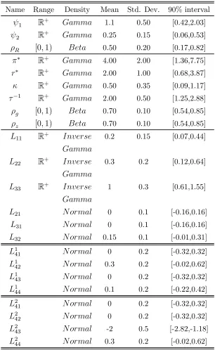
Next, we estimate the parameters of the model on the simulated data and we demonstrate that the posterior estimates of the model parameters are equivalent under two alternative model specifications. Table 1 reports the prior distributions of the parameters used in our estimation. With the ex-ception of priors over the elements of, the prior distributions for the other parameters are the same as in Lubik and Schorfheide (2004)8.
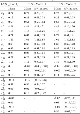
Table 2 compares the posterior estimates of the model parameters. While
the first column reports the parameter values used to simulate the data,
columns two and three are the estimates for two alternative partitions p1
and p2. Partition p1 treats 1 as fundamental and partition p2 treats
2 as fundamental. We used a random walk Metropolis-Hastings algorithm to obtain 150,000 draws from the posterior mean and we report 90-percent probability intervals of the estimated parameters9.
Compare the mean parameter estimates across the three columns. Fifteen of these parameters are common to all three specifications; these are the parameters1 2 ∗ ∗ −1 11 22 33 21 31and32. The
remaining four parameters reported in columns 2 and 3, 41 42 43 and
44 represent the elements of the matrix that are not comparable across
specifications.
8The only difference with respect to Lubik and Schorfheide (2004) is that we use a
flatter prior for the parameter. While the authors set a gamma distribution with mean
05and standard deviation02, our prior sets the standard deviation to035, leaving the mean unchanged. Choosing aflatter prior avoids facing an issue in the convergence of the parameter which arises with a relatively tight prior as in Lubik and Schorfheide (2004). Also, Table 1 reports the mean, the standard deviation and the 90-percent probability interval for each parameter. Note that we were unable to replicate the probability intervals in Lubik and Schorfheide (2004) and we report the 5-th and the 95-th percentiles of each distribution. However, the differences with Lubik and Schorfheide (2004) in the values for the probability intervals are small.
Table 1: Prior Distribution for DSGE Model Parameters
Name Range Density Mean Std. Dev. 90% interval
1 R+ 1.1 0.50 [0.42,2.03]
2 R+ 0.25 0.15 [0.06,0.53]
[01) 0.50 0.20 [0.17,0.82]
∗ R+ 4.00 2.00 [1.36,7.75]
∗ R+ 2.00 1.00 [0.68,3.87]
R+ 0.50 0.35 [0.09,1.17]
−1
R+ 2.00 0.50 [1.25,2.88]
[01) 0.70 0.10 [0.54,0.85] [01) 0.70 0.10 [0.54,0.85]
11 R+ 0.2 0.15 [0.07,0.44]
22 R+ 0.3 0.2 [0.12,0.64]
33 R+ 1 0.3 [0.61,1.55]
21 0 0.1 [-0.16,0.16]
31 0 0.1 [-0.16,0.16]
32 0.15 0.1 [-0.01,0.31]
1
41 0 0.2 [-0.32,0.32]
1
42 0.3 0.2 [-0.02,0.62]
1
43 0 0.2 [-0.32,0.32]
1
44 0.1 0.2 [-0.22,0.42]
2
41 0 0.2 [-0.32,0.32]
2
42 0 0.2 [-0.32,0.32]
2
43 -2 0.5 [-2.82,-1.18]
2
Table 2: Posterior Means and Probability Intervals
L&S (prior 1) FKN - Model 1 FKN - Model 2 Mean Mean 90% interval Mean 90% interval
1 0.77 0.77 [0.73,0.81] 0.77 [0.73,0.81]
2 0.17 0.21 [0.08,0.33] 0.22 [0.08,0.35]
0.60 0.61 [0.59,0.63] 0.61 [0.59,0.63] ∗ 4.28 4.44 [4.17,4.71] 4.43 [4.16,4.70] ∗ 1.13 1.18 [1.10,1.25] 1.17 [1.10,1.25] 0.77 0.67 [0.47,0.89] 0.71 [0.51,0.91] −1 1.45 1.63 [1.41,1.85] 1.61 [1.39,1.82] 0.68 0.66 [0.62,0.70] 0.66 [0.62,0.70] 0.82 0.83 [0.81,0.84] 0.83 [0.81,0.85] 11 0.23 0.23 [0.22,0.24] 0.23 [0.22,0.24]
22 0.27 0.25 [0.21,0.29] 0.25 [0.21,0.29]
33 1.11 1.14 [0.90,1.37] 1.10 [0.87,1.30]
21 0 -0.01 [-0.03,0.009] -0.01 [-0.03,0.009]
31 0 0.02 [-0.09,0.14] 0.003 [-0.09,0.09]
32 0.15 0.14 [0.01,0.27] 0.14 [0.04,0.25]
1
41 -0.14 -0.15 [-0.18,-0.13] -
-1
42 0.37 0.36 [0.34,0.37] -
-143 0.04 0.02 [-0.02,0.07] -
-144 0.10 0.10 [-0.20,0.42] -
-2
41 -0.05 - - -0.07 [-0.25,0.11]
2
42 0.04 - - 0.03 [-0.17,0.22]
2
43 -2.12 - - -2.09 [-2.16,-2.01]
2
44 0.26 - - 0.30 [-0.02,0.62]
probability intervals are statistically indistinguishable when comparing the two alternative models. This correspondence in parameter estimates across specifications is a consequence of Theorems 1 and 2 of our paper.
7
Implementing our Procedure in Dynare
This section provides a practical guide to the user who wishes to implement our method in Dynare. Consider the New-Keynesian model described in Section 6, which we repeat below for completeness,
=[+1]−(−[+1]) + (58)
=[+1] ++ (59)
=−1+ (60)
=−1+ (61)
The model is determinate when monetary policy is active, |1| 1 In this
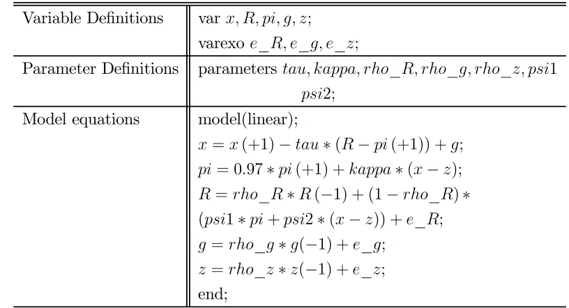
case Dynarefinds the unique series of non-fundamental errors that keeps the state variables bounded and Table 3 reports the code required to estimate the model in this case.
In the case of the indeterminate models described in Section 6.1.2, run-ning Dynare with the code from Table 3 produces an error with a message “Blanchard-Kahn conditions are not satisfied: indeterminacy.” For regions of the parameter space where the code produces that message, we provide two alternative versions of the model that redefine one of the non-fundamental shocks as new fundamental. Following the notation in Section 6.1.2, we refer to these cases as Model 1, where 1=−−1[]is a fundamental shock,
and Model 2, where it is 2 =−−1[]and we present the Dynare code
Table 3: Determinate Model
Variable Definitions var ;
varexo_ _ _;
Parameter Definitions parameters _ _ _ 1
2;
Model equations model(linear);
=(+1)−∗(−(+1)) +;
= 097∗(+1) +∗(−);
=_∗(−1) + (1−_)∗ (1∗+2∗(−)) +_;
=_∗(−1) +_;
=_∗(−1) +_;
end;
Tables 4 and 5 present the amended code for these cases. In Table 4, we show how to change the model by redefining 1 as fundamental and Table 5 presents an equivalent change to Table 3 in which 2 becomes the new fundamental. We have represented the new variables and new equations in that table using bold typeface.
The following steps explain the changes in more detail. First, we define a new variable,xs≡[+1]and include it as one of the endogenous variables
in the model. This leads to the declaration:
xs; (62)
which appears in the first line of Table 4. Next, we add an expectational shock, which we call sunspot, to the set of fundamental shocks, _, _ and _. This leads to the Dynare statement
consumption-Euler equation, which becomes,
=xs−∗(−(+1)) +; (64)
and we add a new equation that defines the relationship between xs, and the new fundamental error:
[image:35.612.109.518.295.543.2]−xs(−1) =sunspot; (65)
Table 4: Indeterminate Model 1: 1 =−−1[] is new fundamental
Variable Definitions var xs;
varexo_ _ _sunspot;
Parameter Definitions parameters _ _ _ 1
2 ;
Model equations model(linear);
=xs−∗(−(+1)) +;
= 097∗(+1) +∗(−);
=_∗(−1) + (1−_)∗ (1∗+2∗(−)) +_;
=_∗(−1) +_;
=_∗(−1) +_;
−xs(−1) =sunspot;
end;
Table 5: Indeterminate Model 2: 2 =−−1[] is new fundamental
Variable Definitions var pis;
varexo_ _ _sunspot;
Parameter Definitions parameters _ _ _ 1
2 ;
Model equations model(linear);
=(+1)−∗(−(+1)) +;
= 097∗pis+∗(−);
=_∗(−1) + (1−_)∗ (1∗+2∗(−)) +_;
=_∗(−1) +_;
=_∗(−1) +_;
−pis(−1) =sunspot;
end;
How can a researcher know, in advance, if his model is determinate. The answer provided by Lubik and Schorfheide (2004), is that determinate and indeterminate models are alternative representations of data that can be compared either by Likelihood ratio tests or by Bayesian model comparison. The Lubik-Schorfheide approach assumes that the researcher can identify, a priori, determinate and indeterminate regions of the parameter space. For models where that is difficult or impossible, Fanelli (2012) and Castelnuovo and Fanelli (2014) propose an alternative method that may be used to test the null hypothesis of determinacy.
8
Conclusion
transforms indeterminate models by redefining a subset of the non-fundamental shocks and classifying them as new fundamentals. Our approach to handling indeterminate equilibria is more easily implementable than that of Lubik and Schorfheide and, one might argue, is also more intuitive. We illustrated our approach using the familiar New-Keynesian monetary model and we showed that, when monetary policy is passive, the new-Keynesian model can be closed in one of two equivalent ways.
A
Appendix A
Proof of Theorem 1. Let 1 and2 be two orthonormal row operators associated with partitions p1 andp2;
⎡ ⎢ ⎣ 1 1 ⎤ ⎥
⎦=1
" # ⎡ ⎢ ⎣ 2 2 ⎤ ⎥
⎦=2
"
#
(A1)
We assume that the operators, have the form
=
⎡
⎣ × 0
0 ˜ ×
⎤
⎦ (A2)
where ˜ is a permutation of the columns of an identity matrix. Pre-multiplying the vector [ ]
by the operator permutes the rows of while leaving the rows of unchanged. Define matrices Ω and Ω for ∈{12}to be the new terms in the fundamental covariance matrix,
⎛ ⎝ " # " #⎞ ⎠= "
Ω Ω Ω Ω
#
Next, use (22) and (23) to write the non-fundamentals as linear functions of the fundamentals,
=Θ+Θ (A3) where
Θ ≡ −³Π˜2´−
1
˜
Ψ2 and Θ ≡ −
³
˜
Π2´−
1
˜
and define the matrix = ⎡ ⎢ ⎢ ⎢ ⎢ ⎣ × 0 × 0 × × Θ (−)× Θ (−)× ⎤ ⎥ ⎥ ⎥ ⎥
⎦ (A5)
Using this definition, the covariance matrix of all shocks, fundamental and non-fundamental, has the following representation,
⎛ ⎜ ⎜ ⎝ ⎡ ⎢ ⎣ ⎤ ⎥ ⎦ ⎡ ⎢ ⎣ ⎤ ⎥ ⎦ ⎞ ⎟ ⎟ ⎠= "
Ω Ω Ω Ω
#
(A6)
We can also combine the last two row blocks of and write as follows
=
⎡ ⎢ ⎣
× ×0 21 × 22 × ⎤ ⎥
⎦ (A7)
where,
21=
⎡ ⎢ ⎣ 0 × Θ (−)× ⎤ ⎥
⎦ 22=
⎡ ⎢ ⎣ × Θ (−)× ⎤ ⎥
⎦ (A8)
Using (A1) and the fact that is orthonormal, we can write the following expression for the complete set of shocks
" # = ⎡ ⎢ ⎣ ⎤ ⎥
Using equations (A6) and (A9), it follows that ⎛ ⎝ " # " #⎞
⎠= for all p ∈P (A10)
where
≡
"
Ω Ω Ω Ω
# (A11) and ≡ = " 0
0 ˜
# "
0
21 22
#
=
"
0
21 22
#
(A12)
Using this expression, we can write out equation (A10) in full to give,
⎛ ⎝ " # " #⎞ ⎠= " 0
21 22
# "
Ω Ω Ω Ω
# "
21
0
22
#
(A13)
We seek to establish that for any partition p, parameterized by matrices Ω and Ω that there exist matrices Ω and Ω for all partitions p ∈ P 6=, such that
Ω= ⎛ ⎝ " # " #⎞
⎠= = (A14)
elements which give three equations in the matrices of Ω andΩ
Ω11 = Ω Ω12 = Ω
21 +Ω22 (A15)
Ω22 = 21 Ω21 + 221Ω22 +22 Ω 22
The first of these equations defines the covariance of the fundamental shocks and it holds for all . Now define
=(Ω) =(Ω) =(Ω ) (A16)
Using the fact that
() =¡ ⊗¢ () (A17)
we can pass theoperator through equation (A15) and write the following system of linear equations in the unknowns and
"
#
+=
"
#
+ (A18)
=
" ¡
22⊗
¢
0
¡
22⊗
21
¢ ¡
22⊗22
¢ #
=
" ¡
21⊗
¢ ¡
21⊗21
¢ #
∈{ }
(A19) It follows from the assumption that the equilibrium is regular that has full rank for all hence for any permutation p parameterized by{ }we can find an alternative permutationp with associated parameterization{
}
"
#
=¡¢−1
Ã
"
#
+£−¤
!
(A20)
non-fundamental shocks.
B
Appendix B
Proof of Lemma 1. We seek to characterize the full set of solutions to the equation,
˜
Ψ2
× ×1
+ ˜Π2
× ×1
= 0 (B1)
Let 1 and11 characterize the singular value decomposition ofΠ˜2
˜ Π2 × ≡ 1 × h 11 × 0 × i
× (B2)
where we partition the matrix as
= ∙ 1 × 2 × ¸
Let characterize a regular indeterminate equilibrium for some partition p and we partition into two mutually exclusive subsets,
and such that
∪ = . From Appendix A, equation A3, we write the non-fundamentals
as functions of the fundamentals and whereΘ andΘ are functions of 1
×1
= Θ ×
×1
+ Θ ×
×1
(B3)
Equation (B3) connects the non-fundamental shocks
to the fundamental shocks£
¤
in the FKN equilibrium. Equation (33) reproduced below as (B4), characterizes the additional equations that define an LS equilibrium,
×1
= 1
×
××1 +×2 ×
×1
+ 2
× ×1
where ≡ −11−1
1 Ψ˜2. To establish the connection between the LS and
FKN representations we split the equations of (B4) into two blocks
×1
= 1 ×
××1+ 2 × × ×1
+2 ×
×1
(B5)
×1
= 1 ×
××1+ 2 × × ×1
+ 2 ×
×1
(B6)
where for = 12, the matrices
and are composed of the row vectors of which, according to partition p, correspond to the non-fundamental shocks included as fundamental,
, and those that are still non-fundamental, .
Using (B3) to replacing in (B5) and combining with (B6)
⎡ ⎣ Θ × ⎤ ⎦
×1
= 1 ×
××1−
⎡ ⎣ Θ × 0 × ⎤ ⎦
×1
+ 2 ×
×
×1
+ 2 ×
×1
(B7) where × ≡ ⎡ ⎢ ⎣ × × ⎤ ⎥ ⎦
Premultiplying (B7) by(
2)
and exploiting the fact that is orthonor-mal, leads to the equation
×
×1
=
××1+××1+ ×1 (B8) where
× ≡
¡
2¢ × ⎡ ⎣ Θ × ⎤ ⎦ ×
and × ≡
¡
2¢ ×
1 ×
×−
¡
Rearranging (B8) and defining
× ≡
×+×
(B10)
gives
×1
= ×
×1
−
× ×1 (B11)
which is the expression we seek.
C
Appendix C
Proof of Theorem 2. Let ={1 2} characterize an FKN
equilib-rium. From (B8), which we repeat below omitting the superscriptto reduce notation,
×
×1
= ××1
+ ×
×1
+ ×1
(C1)
Post-multiplying this equation by
and taking expectations gives
×Ω× = ×Ω× +×Ω× = × Ω× (C2) which represents × linear equations in the × elements of ()
as functions of the elements of , and Ω, (these are functions of 1),
and Ω (these are elements of 2). Applying the operator to (C2), using
the algebra of Kronecker products, and rearranging terms gives the following solution for the parameters (),
()
(×)×1
=
(Ω ⊗)−
1 (×)×(×)
"
(⊗)
(×)×(×)
(Ω )
(×)×1
−(⊗)
(×)×2
(Ω) 2×1
#
Using equation (C3) we can construct an expression for the elements of as functions of 1 and2. Post-multiplying equation (B11) by itself transposed,
and taking expectations, we have
Ω ×
=
×Ω×
×−×Ω×
×−×Ω×
×+×Ω×
× (C4)
= ×Ω
×
×−×Ω× ×
where the last equality is obtained using (C2). The terms on the RHS of (C4) are all functions of the known elements of 1 and2. Since the matrix
Ω is symmetric, this gives ×(+ 1)2 equations that determine the parameters of(Ω). This establishes that every ∈Θ defines a unique parameter vector ∈ Θ. To prove the converse, solve equation (C3) for (Ω ) as a function of 1 and the elements of and apply the
operator to (C4) to solve for(Ω ) in terms of1 and(Ω).
D
Appendix D
To run the simulation of the New-Keynesian model in Lubik and Schorfheide (2004) under indeterminacy, we need to compute the matrices , and . We proceed as follows. First, we apply the QZ decomposition to the representation of the model
Γ0()=Γ1()−1 +Ψ()z+Π()η (D1)
where Γ0(), Γ1(),Ψ()andΠ() are described in Section 3. Let
![Table 4: Indeterminate Model 1: 1 = − −1 [] is new fundamental](https://thumb-us.123doks.com/thumbv2/123dok_us/9503303.455763/35.612.109.518.295.543/table-indeterminate-model-is-new-fundamental.webp)
![Table 5: Indeterminate Model 2: 2 = − −1 [] is new fundamental](https://thumb-us.123doks.com/thumbv2/123dok_us/9503303.455763/36.612.110.527.153.396/table-indeterminate-model-is-new-fundamental.webp)
