go.warwick.ac.uk/lib-publications
Original citation:
Domínguez-García, Virginia, Johnson, Samuel and Muñoz, Miguel A.. (2016) Intervality and
coherence in complex networks. Chaos: An Interdisciplinary Journal of Nonlinear Science, 26
(6). 065308.
Permanent WRAP URL:
http://wrap.warwick.ac.uk/80752
Copyright and reuse:
The Warwick Research Archive Portal (WRAP) makes this work by researchers of the
University of Warwick available open access under the following conditions. Copyright ©
and all moral rights to the version of the paper presented here belong to the individual
author(s) and/or other copyright owners. To the extent reasonable and practicable the
material made available in WRAP has been checked for eligibility before being made
available.
Copies of full items can be used for personal research or study, educational, or not-for profit
purposes without prior permission or charge. Provided that the authors, title and full
bibliographic details are credited, a hyperlink and/or URL is given for the original metadata
page and the content is not changed in any way.
Publisher’s statement:
The following article appeared in Domínguez-García, Virginia, Johnson, Samuel and Muñoz,
Miguel A.. (2016) Intervality and coherence in complex networks. Chaos: An Interdisciplinary
Journal of Nonlinear Science, 26 (6). 065308 and may be found at
http://dx.doi.org/10.1063/1.4953163
A note on versions:
The version presented here may differ from the published version or, version of record, if
you wish to cite this item you are advised to consult the publisher’s version.
Virginia Dom´ınguez-Garc´ıa,1 Samuel Johnson,2and Miguel A. Mu˜noz1 1)
Departamento de Electromagnetismo y F´ısica de la Materia and Instituto Carlos I de F´ısica Te´orica y Computacional. Universidad de Granada. E-18071, Granada, Spain.
2)Warwick Mathematics Institute, and Centre for Complexity Science, University of Warwick, Coventry, CV4 7AL,
United Kingdom.
Food webs – networks of predators and prey – have long been known to exhibit “intervality”: species can generally be ordered along a single axis in such a way that the prey of any given predator tend to lie on unbroken compact intervals. Although the meaning of this axis – identified with a “niche” dimension – has remained a mystery, it is assumed to lie at the basis of the highly non-trivial structure of food webs. With this in mind, most trophic network modelling has for decades been based on assigning species a niche value by hand. However, we argue here that intervality should not be considered the cause but rather a consequence of food-web structure. First, analysing a set of 46 empirical food webs, we find that they also exhibitpredator
intervality: the predators of any given species are as likely to be contiguous as the prey are, but in a different ordering. Furthermore, this property is not exclusive of trophic networks: several networks of genes, neurons, metabolites, cellular machines, airports, and words are found to be approximately as interval as food webs. We go on to show that a simple model of food-web assembly which does not make use of a niche axis can nevertheless generate significant intervality. Therefore, the niche dimension (in the sense used for food-web modelling) could in fact be the consequence of other, more fundamental structural traits, such as trophic coherence. We conclude that a new approach to food-web modelling is required for a deeper understanding of ecosystem assembly, structure and function, and propose that certain topological features thought to be specific of food webs are in fact common to many complex networks.
PACS numbers: 5.65.+b, 87.10.Mn, 89.75.-k, 89.75.Fb, 89.75.Hc
For decades food-web modelling has been based on the idea of a “niche dimension”, according to which the species in an ecosystem are considered to be arranged in a specific order, which is tanta-mount to the existence of a one-dimensional hid-den dimension. This assumption is justified by the empirical observation of a topological feature, exhibited by many food webs to a significant de-gree, called “intervality”. We show here that in-tervality is not necessarily the hallmark of a hid-den niche dimension, but may ensue from other food-web structural properties, such as trophic coherence. In fact, we find instances of networks of genes, neurons, metabolites, cellular machines, airports, and words which exhibit intervality as significant as that of food webs. These results support a new approach to food-web modelling, and suggest that certain features of trophic net-works are relevant for directed netnet-works in gen-eral.
I. INTRODUCTION
Charles Darwin concludedOn the Origin of Species rem-iniscing on his famous entangled bank, “clothed with many plants of many kinds, with birds singing on the bushes, with various insects flitting about, and with worms crawling through the damp earth, [...] so differ-ent from each other, and dependdiffer-ent on each other in so
complex a manner”.1 Charles Elton later developed the concept of a food web – a network of predators and prey – as a description for a community of species,2and in the eighties such systems were among the first to be explicitly modelled as random graphs with specific constraints.3,4 With the advent of ever better ecological data and the explosion of research on complex networks, much work has gone into analysing and modelling the structure of food webs, and its relation to population dynamics and ecosystem function.5–10Not least among the motivations for such research has been an awareness that the sixth mass extinction is under way, and that we must strive to understand ecosystems if we are to protect them.11
Field ecologists apply a variety of techniques to infer the predation links which exist between (and sometimes within) the dozens, or hundreds, of species making up specific ecosystems. The results of such observations are sets of trophic networks, or food webs, which can now be analysed quantitatively, as we go on to do here. A food web with S species can be encoded in an S ×S
adjacency matrix A, such that the element Aij is equal to one if speciesi(the predator) consumes speciesj (its prey), and zero if not. In other words, a food web can be regarded as an unweighted, directed network in which the nodes are species and the directed edges represent predation.
When Joel Cohen first examined a set of such food webs in the seventies, he discovered that they exhibited a topological property which he named intervality: the species could be ordered in a line in such a way that the prey of any given predator would form a compact
interval.4,12In terms of the adjacency matrix, this meant that the columns could be ordered so that elements would form unbroken horizontal blocks (see Figure 1A). This observation re-invigorated the use of an important and old concept in ecology: the niche. The term was origi-nally used simply to refer to a species’ habitat13 or eco-logical role,2 but was then defined by Hutchinson as a “position in a multi-dimensional hyperspace” – each di-mension being some biologically relevant magnitude.14 The observed intervality of food webs suggested that predators consume every species within a particular com-pact hypervolume of niche space – and, moreover, that niche space was (at least to a good approximation) one-dimensional.7,15
Motivated by the belief that complex systems could come about from simple rules, several models were put forward to explain the non-trivial structure of trophic networks. The cascade model was the first such attempt.3 The key idea behind this model is that food webs reflect some inherent hierarchy in which certain species are above others. Hence, species are organised on a hierarchical (niche) axis and are constrained to con-sume only prey which are below them.12The approach is loosely based on the fact that predators tend to be larger than their prey, at least in certain kinds of ecosystem, and so the hierarchy could be regarded as one defined by body size. The cascade model was better at reproduc-ing food-web structure than a fully random graph, but there were features – intervality, in particular – which it could not account for. Then Williams and Martinez put forward the well-known niche model,15 in which species are again ordered along a hierarchical or niche axis, but species are allowed to select prey now only on a contigu-ous interval below them (not a random selection, as in the cascade model). Thus, the niche model has intervality as a built-in property. It also proved quite successful in ex-plaining certain other food-webs properties, and, thanks to its simplicity, it is often taken as the reference model for generating synthetic food webs.16,17 The popularity enjoyed by the niche model has served to reinforce the belief that something akin to its niche axis does in fact form the backbone of real ecosystems.18,19
As progressively better collections of food-web data were gathered, it became apparent that most trophic net-works were not perfectly interval (see Figure 1B). Mea-sures of local “frustration” were proposed to capture the distance from perfect intervality,21and more recently the degree of intervality of food webs has been measured with several continuous quantities that take values close to unity if most of the prey lie on unbroken intervals, or approach zero when very few do.18,19 A simple way is to measure, for each predator, the size of its largest unbro-ken interval as a fraction of its total number of prey, and use the average value over predators as a measure of the intervality – also sometimes called contiguity – ξ of the food web; however, since intervality is defined for a given ordering of species, some optimization method is required to find the most interval global ordering, much as is done
s
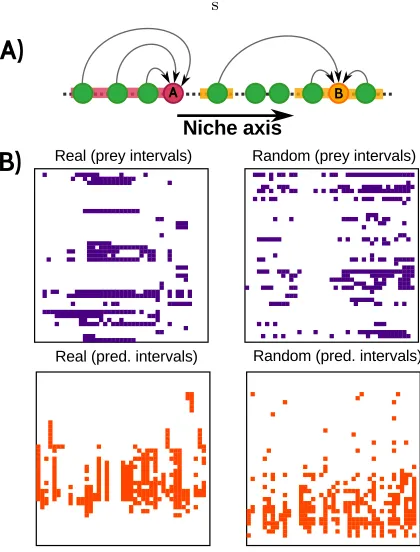
Figure 1. A) Examples of interval and non-interval “diets”. Once species have been arranged along some hidden (niche) axis, species A is said to have an interval diet if all their prey occupy contiguous positions, while species B has a non-interval diet. Different orderings may result in different values of diet intervality for a given predator species. The niche or-dering is defined as the one maximizing the overall level of in-tervality. B) Top left panel: Adjacency matrix corresponding to the empirically obtained food web of Mondego Estuary.20 Filled squares stand for predators (vertical axis) consuming the corresponding prey (horizontal axis); as usual, the same ordering is used for both rows and columns. An ordering of the species has been sought which maximizes prey-intervality,
ξ(see main text for a definition): observe that the prey of any predator tend to be contiguous/interval. Top right panel: The same procedure is applied to a randomised version of the net-work which preserves both in- and out-degree sequences for each node in the Mondego food web; observe the strong reduc-tion in the level of intervality. Bottom left panel: The same adjacency as in the top left panel, but this time according to an ordering or elements which maximises predator-intervality,
η(see main text). Note that this ordering is clearly different from the one found in the panel above. Bottom right panel: Reorganised matrix maximisingη for a network randomisa-tion.
[image:3.612.332.542.51.327.2]ratio-nale is that the imperfect intervality of food webs might be a sign that there are, in fact, more than one niche dimension.25 Despite these developments, some kind of niche axis is still generally thought to underlie food-web structure.
Here, we challenge this view by appealing to three ob-servations.
First, we highlight that predator intervality (the ex-tent to which the predators of a given species can be arranged on unbroken intervals;19i.e. the predator inter-vality of a matrixAis the prey intervality of its transpose,
AT) seems to be as general and non-trivial a feature of food webs asprey-intervality. While it is conceivable that predators might “choose” their prey according to a niche axis, how can prey simultaneously select their predators according to a different ordering?
Second, we show that intervality is not a feature pecu-liar to food webs, as has usually been assumed: complex networks of various kinds – including those of genes, neu-rons, metabolites, cellular machines, airports, and words – exhibit levels of both prey (column) and predator (row) intervality similar to those of food webs. Yet it appears far-fetched to suggest that such diverse systems all owe their structure to some kind of hidden niche axis.
Third, we show that the recently proposed “preferen-tial preying” model of food-web assembly, which does not involve a niche axis, generates significant intervality.26 This is the first model to correctly reproduce the trophic coherence of food webs –i.e. the fact that species can be assigned trophic levels and predators have a tendency to prey upon subsets of prey which are on similar such levels– and we find that a degree of intervality is a by-product of this topological feature. We go on to propose a version of the preferential preying model, amended to take account of phylogenetic constraints, which generates realistic values of intervality without fitting additional parameter values.
Taken together, we believe these observations call into question the concept of a niche dimension, whether as an operationally useful construct for food-web modelling, or as a reality to be uncovered in nature. We conclude by discussing what these findings might mean for our understanding of food-webs and other complex networks.
II. RESULTS
A. Intervality
Let us consider a directed network with S nodes and
L edges, defined by the S ×S adjacency matrix A. As we have said, in the case of a trophic network the nodes are species and the edges represent predation. The in- and out-degrees of node i are kini = P
jAij and
kout
i =
P
jAji, and correspond to the numbers of prey and predators of species i, respectively; and the mean degree ishki=L/S. Basal species, or autotrophs, have no in-coming edges, and are thus represented by nodes
with kin = 0. We shall denote with B the number of basal nodes in a given network.
The top left panel of Fig.1.B shows the adjacency ma-trix for the food web of Mondego Estuary,20 on the At-lantic coast of Portugal, with species ordered so as to maximize intervality ξ (see Methods). Since there are
S! possible orderings of the columns it is not feasible in general to perform an exhaustive search for the most in-terval one. Therefore, we proceed as Stoufferet al.18and use a simulated annealing (SA) algorithm – described in the Methods section. For comparison, in the top right panel of Fig.1.B we show the best ordering for a randomi-sation of the network which preserves kin and kout for each node. These plots readily reveal that the empirical food web is remarkably more interval than its randomised counterpart. Observe, however, that the random network exhibits a non-zero level of intervality, since this magni-tude is defined for the most interval ordering out of a great many possible choices. It is therefore always nec-essary to compare empirical values of intervality to the corresponding random expectations in a null model, in order to determine the significance of this measurement. In the bottom left panel of Fig.1.B we show the same Mondego Estuary adjacency matrix, but this time an ordering has been found which maximises predator-intervality, η: the extent to which the predators of a given prey species are contiguous19 (as above, the same procedure has been applied to an ensemble of network randomisations). The real food web is significantly more predator-interval, while the random graph has some de-gree of predator-intervality (there is a preponderance of vertical intervals). Interestingly, the ordering of maxi-mum predator-intervality is different from the one yield-ing the highest prey-intervality, as is obvious to the naked-eye upon inspection of the two patterns. In fact, we shall see that predator-intervality seems to be as gen-eral and non-trivial a feature of food webs as the oft-cited intervalityξ– which we shall henceforth refer to as prey-intervality, to distinguish the two concepts.
does not seem to be limited to food webs; indeed, almost all the other networks in our database show a similar trend, with levels of both intervalities similar to those observed in food webs.
Since the original observation that food webs tended to be interval, the existence of a hidden “niche dimension” has been assumed to be at the root of this deviation from randomness. However, this explanation fits ill with the fact that food webs and other kinds of network exhibit both prey- and predator- intervality to similar degrees of significance. It would seem, rather, that a more general reason must exist which can account for this topological feature.
B. Trophic coherence
One of the most striking characteristics of food webs – perhaps the first that springs to mind upon contem-plating even a child’s drawing of an ecosystem – is the existence of a trophic structure. At the base there are plants, which are consumed by herbivores, which in turn might be preyed upon by omnivores or primary carni-vores, and so the biomass flows from producers all the way up to top predators. Ecologists quantify the posi-tion of a species in a food web with its trophic level l, such that basal species havel= 1, herbivores l= 2, etc. More generally –following Levine27– one can define the (non-integer) trophic levels in a recursive, self-consistent way: the trophic level of a given species is equal to the average level of its prey plus one unit. That is,
li= 1
kin i
X
j
[image:5.612.71.290.424.608.2]Aijlj+ 1 (1)
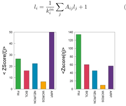
Figure 2. Average z-score for prey (ξ) and predator (η) inter-valities for different type of networks (with respect to a null model consisting in randomisations of each network that pre-serve both kin and kout for each node). Empirical values of
the z-score have been averaged over all networks in each cat-egory. It is evident that empirical values lie well outside the random expectation, with high values of z-scores in all cases. Intervality is therefore a non-trivial feature of many kinds of complex network.
if kiin > 0, or li = 1 if kini = 0. Observe that this definition is easily generalizable to other types of directed network, and each node can be assigned a trophic level by simply solving the set of linear equations given by Eq. (1).28The only requirements for all nodes to have a well-defined level are that there should exist at least one basal node (B >0), and that every non-basal node must be on at least one path including a basal node.29 In fact, this definition of trophic level is similar to other measures of centrality, such as PageRank, with the difference that the “+1” term establishes a natural hierarchy.30
We have recently shown that the trophic structure of a directed network can be characterised by a degree of order we call trophic coherence.26 For this we define a variable x for each edge, as xij = li−lj, and consider the distribution ofxover theLedges of a network. The mean is hxi = 1 by definition, and the homogeneity of the distribution is the trophic coherence of the network. We can therefore quantify this feature simply with the standard deviation ofp(x), which we refer to as an in-coherence parameter: q = phx2i −1. A highly coher-ent network (q '0) is one in which the nodes fall into clear (almost integer) trophic levels, while a more ran-dom system is less coherent (q > 0). We have shown that trophic coherence is key to the linear stability of food webs and, since it can invert the usually positive re-lationship between diversity and stability, might be the solution to Robert May’s famous paradox.26,31,32Trophic coherence has subsequently been found to play an impor-tant role in directed networks of many kinds, including those of neurons, genes, metabolites, cellular signalling, words, P2P, trade and transportation, and this feature is intimately related to cycles and feedback loops, graph eigenspectra and the ubiquity of ‘qualitatively stable’ systems.28,29 Elsewhere in this issue, Klaise & Johnson show that trophic coherence also determines the extent and duration of spreading processes such as epidemics or neuronal cascades.33
Networks with tunable trophic coherence can be gen-erated with the recently proposed preferential preying model(PPM),26 which works as follows. We begin with
B initial nodes (basal species) and no edges. New nodes (consumer species) are added sequentially to the system until a total of S nodes is reached. When a node en-ters the system its in-neighbours (prey) are awarded from among available nodes (those already in the network) in the following way: the first prey species is chosen ran-domly, and the rest are chosen with a probability that decays exponentially with the absolute trophic distance to their initial prey (i.e. with the absolute difference of trophic levels between its first prey and the subsequent ones). This probability is set by a parameter T that determines the degree of trophic specialization of con-sumers, and normalised so as to produce an expected number of edges L. The lower the value of T (while
at consuming species X, then its other prey are likely to have similar trophic levels to that of X, as is observed in nature.34
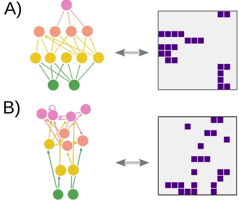
Food webs tend to be very significantly coherent, and this is key to their stability and other properties. How-ever, niche-based models are not able to reproduce this feature, and generate networks which are barely more coherent than random graphs.26 This shows that inter-vality is not a sufficient condition for trophic coherence. Is it possible, though, that trophic coherence induces in-tervality? Figure 3A displays an example of a maximally coherent network (q= 0), obtained with a low T, while figure 3B is an instance of a less coherent network (q >0), obtained with a high T (see also Fig.4). Beside each of them appears its adjacency matrix, where species have been ordered in such a way as to maximise prey interval-ity,ξ. The maximally coherent network is also perfectly interval, while the incoherent one has gaps which cannot be eliminated by changing the arrangement of nodes in any way. This trend is more clearly illustrated in Fig.4, which shows that both prey- and predator-intervalities decrease monotonically withT.
[image:6.612.58.293.435.635.2]For an intuitive understanding of why intervality emerges in the presence of trophic coherence, imagine a simple food web consisting only of na predators that prey upon a different set of nb species. It will be more likely that there is an ordering of the prey such thatξis high –or one of predators such thatηis– ifna andnb are small (i.e. if the adjacency matrix contains few rows and columns). If a food web is perfectly stratified (q = 0) so that species on levell are only consumed by those on
Figure 3. A: Network generated with the preferential preying model (PPM) withS = 12,B = 2 andT = 0 (the vertical position of each node reflects its trophic level) and its corre-sponding adjacency matrix, with rows and columns ordered to maximize prey-intervality (ξ= 1). B: As A but for a similar randomised network, leading to a smaller intervalityξ= 0.90.
levell+ 1, then the network can be seen as a superposi-tion of many of these (independent) simple situasuperposi-tions (A
will have a “modular” or block structure). Given that at each pair of levels the number of species is significantly smaller than the total numberS, a global ordering can be found yielding as good aξas in the simple example – or a different ordering for as good anη. Networks that are thus highly coherent will have higher values of both intervalities than those lacking this structure.
C. Topological features contributing to Intervality
The reasoning described above suggests that trophic co-herence should not be the only feature related to inter-vality. Indeed, as illustrated below, trophic coherence can only account for a fraction of the total intervality observed in empirical networks.
In general, any property which had the effect of cre-ating modularity –i.e. de-coupling certain non-zero ma-trix elements from others, in the sense that their rows or columns could be shuffled without affecting the ordering of other elements– would be conducive to higher levels of intervality. In other words, we should expect a high prey-intervality in networks in which nodes sharing any in-neighbours tended to share a high proportion of them; and the same goes for predator-intervality and shared out-neighbours. To capture this feature, we can define
in-complementarity cin as the mean number of shared neighbours over all pairs of nodes with any shared in-neighbours; and, similarly, out-complementarity cout as the mean number of shared out-neighbours over all pairs of nodes with any shared out-neighbours.
We have measured the relationships between inter-vality and several topological properties (including S,
hki, q and complementarities cin and cout). The cor-relation between ξ and cin has a Pearson coefficient of
r = 0.83, precisely the same as that of η and cout. In other words, complementarity –i.e. the proportions of shared in-neighbours and of shared out-neighbours– ac-counts for approximately 70% of the variance in prey- and predator-intervalities, respectively, across a broad range of empirical networks. The correlations with trophic co-herence itself are lower but still significant (r ≈ 0.55). The mean degree, hki, and the number of nodes, S, are both negatively correlated with both kinds of intervality (r ≈ −0.67 and r ≈ −0.45, respectively), as we would expect from the reasoning above.
D. Modelling networks with coherence and intervality
0.2 0.4 0.6 0.8
0 1 2 3 4 5 q
T
0.85 0.9 0.95 1
0 1 2 3 4 5 ξ
T
0.8 0.85 0.9 0.95
0 1 2 3 4 5 η
[image:7.612.60.550.54.162.2]T
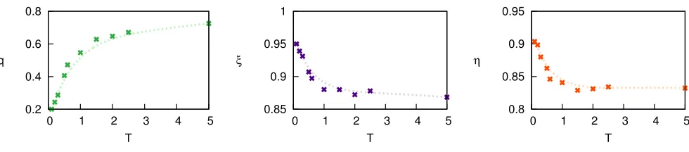
Figure 4. Left panel: Incoherence parameterqas a function of the tunable parameterT as obtained in thepreferential preying model(PPM)26(N = 31L= 68 as in the Chesapeake bay food web35,36). For eachT, the reported values (crosses) are averages over 100 independent network realisations. AsT increases the generated networks are more incoherent. The Central (Right) panel shows prey (predator) intervalityξ(η), as measured in the same networks. Discontinuous lines are just interpolations.
istence of phylogenetic relationships between species – i.e. of common ancestry – was not modelled as a niche axis, but as a “diet overlap” for certain pairs of species. The thinking is that species which are closely related to each other (phylogenetically similar) will tend to share many of their prey. Cattin and colleagues found that phylogenetic constraints, modelled in this way, increase intervality21 – and subsequent empirical work has rein-forced this connection.38,39 These results are in keeping with the view that any mechanism with the effect of mak-ing nodes topologically similar (such as close relatives having many shared prey or predators, in the case of food webs) will also lead to seemingly non-random levels of intervality. But since topologically similar nodes can exist for many different reasons, it is not just food webs which exhibit intervality, but directed networks of many different kinds.
In the case of food webs, we know that both trophic coherence and a phylogenetic signal are present. To plore whether these properties might be sufficient to ex-plain the observed intervality, we extend the PPM to ac-count for the effect of phylogenetic relations in a simple parameter-free way. For this we draw inspiration from the “nested hierarchy” model of Cattinet al.,21 and de-fine a version of the PPM in which new nodes are assigned in-neighbours (prey) according not only to their trophic levels, as before, but also with a preference for nodes which already share out-neighbours (predators) when-ever possible (see Methods for a detailed description of this model). Figure 5 illustrates the performance of this modified PPM model compared to its original version for the Chesapeake bay food web. In particular, we generate networks with the modified model fixingN, LandB as in the empirical network, and choose the optimal value of T (vertical dashed line) that leads to a value ofq as close as possible to the empirical one (horizontal dotted line in Fig. 5). For this same value of T, the obtained intervalityξfits quite well with its empirical counterpart (z-score−0.22).
Observe, that while the dependence of the incoherence parameter, q, on the only parameter, T, remains as in
the original version, the intervalityξ obtained with the modified model is higher and much closer to the empir-ical value. Similar results are obtained, in general, for other trophic networks (e.g. for Narragan bay the z-score is−0.43, for St. Marks −1.06, and for St. Martin
−0.89), while a few exceptions exist (e.g. for the Ever-glades marshes we obtain−6.52, indicating that in this case our model does not account for the observed vality). Worse agreement is obtained for predator inter-vality η; in the example of Figure 5, the corresponding z-score is−2.04. The reason for this is that intervality is strongly influenced by the degree sequences (see the def-initions ofξ and η) and the PPM model –as well as its modified variant– fit the empirical in-degree distribution, but not the out-degree one, which is the one affectingη
the most.
The justification for the proposed combination of trophic specialization and phylogenetic relations has a clear meaning only in the case of food webs. We leave as an open question to determine which mechanisms akin to these ones are at work in systems other than food webs, or whether there are different mechanisms which have a similar effect on intervality.
III. DISCUSSION
Figure 5. Figure analogous to Fig. 4 for the Chesapeake Bay food web,35,36 but employing the modified –rather than the
original– version of the PPM, which includes a preference to choose prey which already share some predators (or prey). Results for the original PPM are also reported (light colors) for the sake of comparison. Dotted horizontal lines indicate the empirical values as measured in the real food web, while vertical ones stand for the value ofT providing the best fit toq. Observe that, while trophic coherence is not significantly changed by this modification to the model, the levels of intervality (ξ and η) are clearly augmented by the effect of a phylogenetic signal and become closer to the real values.
the niche model.7,16,21,24,25Going on this, attempts have been made to identify the niche axis with some biological magnitude, such as body size, but no such measure has ever been found to align completely with the orderings of maximum intervality.19,44 It is worth noting that Ross-berg et al.45 were able to generate interval networks in anN-dimensional niche space provided phylogenetic re-lationships were present, thus proving that, contrary to general belief, a one-dimensional space was not a neces-sary condition for the emergence of intervality. In their model species evolution is represented as a random walker in theN-dimensional niche space, and over time species can go extinct or speciate into new ones. As long as new species are close to the parent ones in niche space, the resulting networks are highly interval.
We propose here that the intervality of food webs does not justify invoking hidden or niche dimensions. We have shown that food webs exhibit as much predator-intervality as prey-predator-intervality, which seems incompatible with the interpretation of niche-based models. Moreover, we find that many different kinds of biological and arti-ficial networks are as significantly interval as food webs. This means that either these various networks were all as-sembled according to the stringent constraints of a niche-axis analogue –which appears highly unlikely– or signif-icant intervality need not be the hallmark of hidden di-mensions. The latter explanation is further supported by the strong correlation between intervality and the aver-age proportion of shared neighbours (complementarity) found across all networks. Finally, a one-parameter, en-tirely niche-free network model, based on the “prefer-ential preying”26 and the “nested hierarchy”21 models, which emulates trophic specialization and phylogenetic relations, yields similar levels of intervality as those ob-served in food webs and other networks.
There are two messages to be drawn from this pa-per. For ecologists, we cannot say whether our results should change the interpretation of the niche concept more broadly, but as regards food-web modelling we be-lieve the case is clear for a new approach. The niche axis –like Ptolemy’s epicycles, phlogiston, caloric,
luminifer-ous aether, and other constructs eventually found lacking in empirical support– should be abandoned. This does not mean that Williams & Martinez’s idea of food-web complexity arising from simple rules is wrong, only that we must update our concepts of these rules.
For the study of complex networks more generally, these results show that there are still open questions about the basic mechanisms behind their formation. Shared neighbours explain 70% of the variance in inter-vality, but whence the rest? Do other properties induce such apparent order, or are there, after all, hidden hier-archies underlying the architectures of certain complex systems?28,46 The high significance of topological prop-erties such as intervality and trophic coherence found in many different kinds of system, from neural networks to trading relations, and word graphs to gene regulatory networks, suggests that we, like Darwin admiring the complexity of his entangled bank, have yet much to learn from ecosystems.
IV. METHODS
Measuring intervality.Given a food web and a specified order-ing of speciesO, we define the prey-intervality,ξOi , of each predator speciesias the largest number of its prey to lie on an unbroken interval divided by the total number of prey it has. The prey-intervality of the ordering is then the average over all predator species of this value,ξO = 1
N−B
P
iξOi . The prey-intervality of the food web itself is defined as that of the ordering with the high-est prey-intervality:ξ= max{ξO}O. Given that the search cannot be made exhaustively, we implement a standard simulated anneal-ing algorithm. For this, one begins with a random orderanneal-ingO1and measures its prey-intervalityξO1; then two species are randomly chosen and their positions in the ordering exchanged, yielding a new orderingO2. The new prey-intervalityξO2 is calculated; and the permutation is accepted with probability
P1→2= min
exp
ξO2−ξO1
p
,1
,
for each measurement. In all cases, the algorithm converges to a unique value of ξ for a given network. The predator-intervality,
η, is obtained in an analogous way. Observe that this measure is slightly different from the one defined by Stoufferet al.,18 which is based on the “generalized niche model”; but both measures are strongly correlated (we have found a Pearson’s coefficientr= 0.82 between the two measurements over our network dataset).
Measuring complementarity. Given a food web we define its matrix of shared prey as M = AAT, where A is the adja-cency matrix. The elementmij is the number of prey that are shared by speciesi andj. Similarly, the matrix of shared preda-tors is ˆM = ATA. The in-complementarity between i and j is defined aswij = mij/max(kiin, kinj ), and similarly, for the out-complementarity ˆwij = ˆmij/max(kouti , kjout). By averaging over all possible pairs with at least one common shared in/out neigh-bour, we determine the overall complementarities cin and cout, respectively.
Modified Preferential preying model with phylogenetic constraints.The original preferential preying model was designed to generate networks with tunable trophic coherence. Here we in-troduce an additional mechanism implementing the idea that a predator is likely to choose prey which are similar, i.e. that share other predators or other prey. In the standard PPM one starts with
Bbasal nodes and adds progressively new species, up to a total of
S. Each one selects its prey from existing network nodes, following these rules: i) The in-degree (kin) of species iis selected from a Beta distribution, so as to obtain on average the same number of linksLas the empirical network to be modelled. ii) The first prey species (l) is randomly selected from the available ones. iii) Subse-quent prey (j) are chosen with a probabilityPilthat decays with the trophic distance betweenjandl:
Pil∼exp(− |sj−sl|
T ),
where T is a “temperature” parameter that sets the degree of trophic specialization. In this version of the PPM, in order to in-clude an additional preference for phylogenetically related species as done by Cattinet al.21, we modify rule iii) as follows. First we chose a preyjas above and consider all other possible prey with the same trophic level (plus/minus 1%) and from this group we randomly select one among the subgroup that already has some predator with any of the existing prey ofi. If there is no species obeying these constraints, thenjis selected.
ACKNOWLEDGMENTS
Acknowledgments –We acknowledge the Spanish-MINECO grant FIS2013-43201-P (FEDER funds) for financial support.
REFERENCES
1C. Darwin,On the Origin of Species(John Murray, London,UK, 1859).
2C. S. Elton, Animal Ecology (Sidgwick and Jackson, London, 1927).
3J. E. Cohen and C. M. Newman, “A stochastic theory of com-munity food webs I. models and aggregated data,” Proc. R. Soc. London Ser. B.224, 421–448 (1985).
4J. E. Cohen,Food Webs and Niche Space(Princeton Univ. Press, Princeton, New Jersey, 1978).
5S. L. Pimm,The Balance of Nature? Ecological Issues in the Conservation of Species and Communities (The University of Chicago Press, Chicago, 1991).
6B. Drossel and A. J. McKane,Modelling Food Webs, in A Hand-book of Graphs and Networks: From the Genome to the Internet
(Wiley-VCH, Berlin, 2003).
7J. A. Dunne,The network structure of food webs, in Ecological Networks: Linking Structure to Dynamics in Food Webs, edited by M. Pascual and e. J.A. Dunne (Oxford University Press, Ox-ford, UK, 2006).
8R. V. Sol´e and J. Bascompte, Self-Organization in Complex Ecosystems(Princeton University Press, Princeton, USA, 2006). 9J. Camacho, R. Guimer´a, and L. A. N. Amaral, “Robust patterns
in food web structure,” Phys. Rev. Lett.88, 228102 (2002). 10R. V. Sol´e and M. Montoya, “Complexity and fragility in
ecolog-ical networks,” Proc. R. Soc. Lond. B268, 2039204 (2001). 11J. M. De Vos, L. N. Joppa, J. L. Gittleman, P. R. Stephens, and
S. L. Pimm, “Estimating the normal background rate of species extinction,” Conservation Biology29, 452–462 (2015).
12J. E. Cohen, “Food webs and the dimensionality of trophic niche space,” Proc. Natl. Acad. Sci. USA74, 4533–4563 (1977). 13J. Grinnell, “The niche-relationships of the California Thrasher,”
Auk34, 427–433 (1917).
14G. E. Hutchinson, “Concluding remarks,” Cold Springs Harbor Symp. Quant. Biol.22, 415–427 (1957).
15R. J. Williams and N. D. Martinez, “Simple rules yield complex food webs,” Nature404, 180–183 (2000).
16R. J. Williams and N. D. Martinez, “Success and its limits among structural models of complex food webs,” Journal of Animal Ecol-ogy77, 512–519 (2008).
17C. Guill and B. Drossel, “Emergence of complexity in evolv-ing niche-model food webs,” Journal of Theoretical Biology251, 108120 (2008).
18D. B. Stouffer, J. Camacho, and L. A. N. Amaral, “A robust measure of food web intervality,” Proc. Natl. Acad. Sci. USA
103, 19015–19020 (2006).
19A. E. Zook, A. Ekl¨of, U. Jacob, and S. Allesina, “Food webs: Ordering species according to body size yields high degree of intervality,” Journal of Theoretical Biology271, 106–113 (2011). 20J. Patricio, “Network analysis of trophic dynamics in south florida ecosystems, fy 99: The graminoid ecosystem.” Master’s Thesis. University of Coimbra, Coimbra, Portugal (2000). 21M. F. Cattin, L. F. Bersier, C. Banasek-Richter, R.
Bal-tensperger, and J. P. Gabriel, “Phylogenetic constraints and adaptation explain food-web structure,” Nature 427, 835–9 (2004).
22M. Girvan and M. E. J. Newman, “Community structure in social and biological networks,” Proc. Natl. Acad. Sci. USA99, 7821– 7826 (2002).
23S. Johnson, V. Dom´ınguez-Garc´ıa, and M. A. Mu˜noz, “Fac-tors determining nestedness in complex networks,” PloS ONE8, e74025 (2013).
24D. B. Stouffer, J. Camacho, R. Guimer`a, C. A. Ng, and L. A. N. Amaral, “Quantitative patterns in the structure of model and empirical food webs,” Ecology86, 13011311 (2005).
25S. Allesina, D. Alonso, and M. Pascual, “A general model for food web structure,” Science320, 658–661 (2008).
26S. Johnson, V. Dom´ınguez-Garc´ıa, L. Donetti, and M. A. Mu˜noz, “Trophic coherence determines food-web stability,” Proc. Natl. Acad. Sci. USA111, 17923–17928 (2014).
27S. Levine, “Several measures of trophic structure applicable to complex food webs,” J. Theor. Biol.83, 195–207 (1980). 28V. Dom´ınguez-Garc´ıa, S. Pigolotti, and M. A. Mu˜noz, “Inherent
directionality explains the lack of feedback loops in empirical networks,” Scientific Reports4, 7497 (2014).
29S. Johnson and N. S. Jones, “Spectra and cycle structure of trophically coherent graphs,” arXiv:1505.07332 (2015). 30V. Dom´ınguez-Garc´ıa and M. A. Mu˜noz, “Ranking species in
mutualistic networks,” Scientific reports5(2015).
31R. M. May, “Will a large complex system be stable?” Nature
238, 413 (1972).
32K. S. McCann, “The diversity-stability debate,” Nature 405, 228–33 (2000).
34This is the model we use to generate coherent networks in this work; however, we note that Klaise & Johnson33 propose a slightly different version of the PPM, the main difference be-ing that at highT their model limits in random graphs instead of acyclic cascade model networks.
35R. E. Ulanowicz and D. Baird, “Nutrient controls on ecosystem dynamics: the chesapeake mesohaline community,” Journal of Marine Systems19, 159 – 172 (1999).
36L. G. Abarca-Arenas and R. E. Ulanowicz, “The effects of tax-onomic aggregation on network analysis,” Ecological Modelling
149, 285 – 296 (2002).
37J. Capit´an, A. Arenas, and R. Guimer´a, “Degree of interval-ity of food webs: From body-size data to models,” Journal of Theoretical Biology334, 35–44 (2013).
38A. Ekl¨of and D. B. Stouffer, “The phylogenetic component of food web structure and intervality,” Theor Ecol (2015). 39D. Mouillot, B. Krasnov, and R. Poulin, “High intervality
ex-plained by phylogenetic constraints in host-parasite webs,” Ecol-ogy89(7), 20432051 (2008).
40G. E. Hutchinson,An Introduction to Population Biology (Yale Univ Press, New Haven, CT, USA., 1978).
41R. K. Colwell and T. F. Rangel, “Hutchinson’s duality: The once and future niche,” Proc. Natl. Acad. Sci. USA106, 19651 (2009). 42G. McInerny and R. Etienne, “Ditch the niche is the niche a useful concept in ecology or species distribution modelling?” J. Biogeogr.39, 20962102 (2012).
43G. McInerny and R. Etienne, “Pitch the niche taking responsi-bility for the concepts we use in ecology and species distribution modelling,” J. Biogeogr.39, 21122118 (2012).
44D. B. Stouffer, E. L. Rezende, and L. A. N. Amaral, “The role of body mass in diet contiguity and food-web structure,” J. Anim. Ecol.80, 632–639 (2011).
45A. G. Rossberg, A. Br¨annstr¨om, and U. Dieckmann, “Food-web structure in low- and high-dimensional trophic niche spaces,” Journal of The Royal Society Interface (2010).
46B. Corominas-Murtra, J. Go˜ni, R. V. Sol´e, and C. Rodrguez-Caso, “On the origins of hierarchy in complex networks,” Proc. Natl. Acad. Sci. USA103, 1331613321 (2013).
47N. G. Jaarsma, S. M. de Boer, C. R. Townsend, R. M. Thomp-son, and E. D. Edwards, “Characterising foodwebs in two new zealand streams,” New Zealand Journal of Marine and Freshwa-ter Research32, 271–286 (1998).
48R. M. Thompson and C. R. Townsend, “Energy availability, spa-tial heterogeneity and ecosystem size predict food-web structure in stream,” Oikos108, 137148 (2005).
49R. M. Thompson, E. D. Edwards, A. R. McIntosh, and C. R. Townsend, “Allocation of effort in stream food-web studies: the best compromise?” Marine and Freshwater Research52, 339345 (2001).
50R. E. Ulanowicz, C. Bondavalli, and M. Egnotovich., “Spatial and temporal variation in the structure of a freshwater food web,” Network Analysis of Trophic Dynamics in South Florida Ecosys-tem, FY 97: The Florida Bay Ecosystem..
51J. G. Field, R. J. M. Crawford, P. A. Wickens, C. L. Moloney, K. L. Cochrane, and C. A. Villacast´ın-Herrero,Network analysis of Benguela pelagic food webs (Benguela Ecology Programme, Workshop on Seal-Fishery Biological Interactions. University of Cape Town, 16-20, September, BEP/SW91/M5a, University of Cape Town, 1991).
52P. Yodzis, “Local trophodynamics and the interaction of marine mammals and fisheries in the Benguela ecosystem,” J. Anim. Ecol.67, 635–658 (1998).
53K. Havens, “Scale and structure in natural food webs,” Science
257, 1107–1109 (1992).
54J. Memmott, N. D. Martinez, and J. E. Cohen, “Predators, parasitoids and pathogens: species richness, trophic generality and body sizes in a natural food web,” J. Anim. Ecol.69, 1–15 (2000).
55C. R. Townsend, R. M. Thompson, A. R. McIntosh, C. Kilroy, E. Edwards, and M. R. Scarsbrook, “Disturbance, resource
sup-ply, and food-web architecture in streams,” Ecol. Let.1, 200–209 (1998).
56J. Bascompte, C. Meli´an, and E. Sala, “Interaction strength combinations and the overfishing of a marine food web,” 102, 5443–5447 (2005).
57K. D. Lafferty, R. F. Hechinger, J. C. Shaw, K. L. Whitney, and A. M. Kuris, “Food webs and parasites in a salt marsh ecosys-tem,” Disease ecology: community structure and pathogen dy-namics (ed. S. Collinge & C. Ray) , 119–134 (2006).
58R. E. Ulanowicz, “Growth and development: Ecosystems phe-nomenology. springer, new york. pp 69-79.” Network Analysis of Trophic Dynamics in South Florida Ecosystem, FY 97: The Florida Bay Ecosystem. (1986).
59R. B. Waide and W. B. Reagan, The Food Web of a Tropical Rainforest (University of Chicago Press, Chicago, 1996). 60R. E. Ulanowicz, J. Heymans, and M. Egnotovich, “Network
analysis of trophic dynamics in south florida ecosystems,” Net-work Analysis of Trophic Dynamics in South Florida Ecosystems FY 99: The Graminoid Ecosystem. (2000).
61N. D. Martinez, B. A. Hawkins, H. A. Dawah, and B. P. Fei-farek, “Effects of sampling effort on characterization of food-web structure,” Ecology80, 10441055 (1999).
62N. D. Martinez, “Artifacts or attributes? Effects of resolution on the Little Rock Lake food web,” Ecol. Monogr.61, 367–392 (1991).
63J. Riede, U. Brose, B. Ebenman, U. Jacob, R. Thompson, C. Townsend, and T. Jonsson, “Stepping in Elton’s footprints: a general scaling model for body masses and trophic levels across ecosystems,” Ecology Letters14, 169–178 (2011).
64A. Ekl¨of, U. Jacob, J. Kopp, J. Bosch, R. Castro-Urgal, B. Dals-gaard, N. Chacoff, C. deSassi, M. Galetti, P. Guimaraes, S. Lom-scolo, A. Martn Gonzlez, M. Pizo, R. Rader, A. Rodrigo, J. Tylianakis, D. Vazquez, and S. Allesina, “The dimensionality of ecological networks,” Ecology Letters16, 577–583 (2013). 65R. E. Ulanowicz, C. Bondavalli, and M. Egnotovich., “Spatial
and temporal variation in the structure of a freshwater food web,” Network Analysis of Trophic Dynamics in South Florida Ecosys-tem, FY 97: The Florida Bay Ecosystem. (1998).
66D. Mason, “Quantifying the impact of exotic invertebrate in-vaders on food web structure and function in the great lakes: A network analysis approach,” Interim Progress Report to the Great Lakes Fisheries Commission- yr 1 (2003).
67M. E. Monaco and R. E. Ulanowicz, “Comparative ecosystem trophic structure of three u.s mid-atlantic estuaries,” Marine Ecology Progress Series161, 239–254 (1997).
68S. Opitz, “Trophic interactions in Caribbean coral reefs,” ICLARM Tech. Rep.43, 341 (1996).
69J. Link, “Does food web theory work for marine ecosystems?” Mar. Ecol. Prog. Ser.230, 1–9 (2002).
70P. H. Warren, “Spatial and temporal variation in the structure of a freshwater food web,” Oikos55, 299–311 (1989).
71R. R. Christian and J. J. Luczkovich, “Organizing and under-standing a winter’s Seagrass foodweb network through effective trophic levels,” Ecol. Model.117, 99–124 (1999).
72L. Goldwasser and J. A. Roughgarden, “Construction of a large Caribbean food web,” Ecology74, 1216–1233 (1993).
73U. Jacob, A. Thierry, U. Brose, W. Arntz, S. Berg, T. Brey, I. Fetzer, T. Jonsson, K. Mintenbeck, C. Mllmann, O. Petchey, J. Riede, and J. Dunne, “The role of body size in complex food webs,” Advances in Ecological Research45, 181–223 (2011). 74S. J. Hall and D. Raffaelli, “Food-web patterns: lessons from a
species-rich web,” J. Anim. Ecol.60, 823–842 (1991).
75J. Duch and A. Arenas, “Community identification using ex-tremal optimization,” Physical Review E72, 027104 (2005). 76J. Sanz, J. Navarro, A. Arbus, C. Martn, P. C. Marijun, and
Y. Moreno, “The transcriptional regulatory network of mycobac-terium tuberculosis,” PLoS ONE6, e22178 (2011).
77H. Yu and M. Gerstein, Proc. Natl. Acad. Sci. USA.
dynamic stability in biological and engineered networks,” PNAS
105, 19235–19240 (2008).
79C. Rodrguez-Caso, B. Corominas-Murtra, and R. V. Sol, “On the basic computational structure of gene regulatory networks,” Mol. BioSyst.5, 1617–1629 (2009).
Name S < k > Type ξZ-score ηZ-score ref Food webs
Akatore Stream 85 2.67 Stream 2.650 (**) 685.250 (***) 47–49 Florida Bay (dry season) 122 14.75 Marine 68.536 (***) 49.307 (***) 50 Florida Bay (wet season) 122 14.48 Marine 55.779 (***) 49.175 (***) 50
Benguela Current 29 7.00 Marine 11.492 (***) 7.028 (***) 51,52 Berwick Stream 79 3.04 Stream 9.206 (***) 6.566 (***) 47–49 Blackrock Stream 87 4.31 Stream 6.350 (***) 6.297 (***) 47–49 Bridge Brook Lake 25 4.28 Lake 14.676 (***) 73.785 (***) 53
Broad Stream 95 5.95 Stream 15.423 (***) 8.742 (***) 47–49 Scotch Broom 85 2.62 Terrestrial 10.644 (***) 23.209 (***) 54 Canton Creek 102 6.83 Stream 13.678 (***) 20.675 (***) 55 Caribbean (2005) 249 13.31 Marine 32.603 (***) 54.878 (***) 56 Carpinteria Salt Marsh Reserve 128 4.23 Marine 24.123 (***) 23.272 (***) 57
Catlins Stream 49 2.24 Stream 4.751 (***) 0.238 () 47–49 Cayman Islands 261 14.43 Marine 52.739 (***) 34.324 (***) 56 Chesapeake Bay 31 2.19 Marine 7.997 (***) 4.868 (***) 35,36 Crystal Lake (control) 20 2.55 Lake 5.454 (***) 15.001 (***) 58
Crystal Lake (delta) 20 1.65 Lake 2.226 (**) 4.405 (***) 58 Cuba 261 14.84 Marine 61.826 (***) 28.068 (***) 56 Cypress (dry season) 65 6.89 Terrestrial 18.791 (***) 187.024 (***) 50 Cypress (wet season) 65 6.75 Terrestrial 25.329 (***) 251.612 (***) 50 Dempsters Stream (autum) 86 4.83 Stream 10.116 (***) 42.483 (***) 47–49
El Verde Rainforest 155 9.74 Terrestrial 56.909 (***) 110.125 (***) 59 Everglades Graminoid Marshes 63 9.79 Terrestrial 51.266 (***) 16.429 (***) 60 Florida Bay 122 14.48 Marine 55.670 (***) 276.139 (***) 50 Graminoid Marshes (dry) 63 9.79 Terrestrial 51.266 (***) 16.429 (***) 60 Graminoid Marshes (wet) 63 9.79 Terrestrial 51.266 (***) 16.429 (***) 60 Grassland 61 1.59 Terrestrial 2.917 (**) 3.516 (***) 61 Healy Stream 96 6.60 Stream 11.242 (***) 67.238 (***) 47–49
Jamaica 263 15.61 Marine 82.760 (***) 179.738 (***) 56 Kyeburn Stream 98 6.42 Stream 8.142 (***) 65.368 (***) 47–49 Little Rock Lake 92 10.84 Lake 54.022 (***) 215.878 (***) 62
Lough Hyne 349 14.66 Marine 67.464 (***) 645.370 (***) 63,64 Mangrove Estuary (dry season) 91 12.63 Marine 36.641 (***) 21.644 (***) 65 Mangrove Estuary (wet season) 91 12.65 Marine 36.163 (***) 77.527 (***) 65 Michigan Lake 35 3.69 Lake 24.402 (***) 36.655 (***) 66 Mondego Estuary 42 6.64 Marine 13.237 (***) 11.951 (***) 20 Narragansett Bay 31 3.65 Marine 6.841 (***) 28.552 (***) 67 Caribbean Reef 50 11.12 Marine 11.179 (***) 2862.490 (***) 68 N.E. Shelf 79 17.76 Marine 24.212 (***) 27.151 (***) 69 Skipwith Pond 25 7.88 Lake 2.504 (**) 15.742 (***) 70 St. Marks Estuary 48 4.60 Marine 21.388 (***) 22.591 (***) 71 St. Martin Island 42 4.88 Terrestrial 12.730 (***) 17.923 (***) 72 Stony Stream 109 7.61 Stream 13.525 (***) 10.515 (***) 55
Troy Stream 78 2.32 Stream 5.686 (***) 6.622 (***) 47–49 Weddell Sea 483 31.81 Marine 120.062 (***) 517.488 (***) 73 Ythan Estuary 82 4.82 Marine 7.713 (***) 21.531 (***) 74
Biological
C. Elengans metabolic 453 4.50 TRN 7.726 (***) 125.040 (***) 75 E. Coli transcription 1037 2.59 TRN 51.538 (***) 78.798 (***) 76 Mus musculus transcription 73 1.62 TRN 3.908 (***) 17.283 (***) 77 Mammalian signalling 599 2.34 Cell signalling 21.686 (***) 43.677 (***) 78 B. Subtilis transcription 814 1.69 TRN 2.305 (**) 85.051 (***) 79 M. Tuberculosis transcription 1624 1.98 TRN -9.637 (***) 11.029 (***) 76
Other Networks
C. Elegans neural 297 7.90 neural 22.429 (***) 45.026 (***) 80 Word adjacency 50 2.02 words 6.479 (***) 9.589 (***)
[image:12.612.133.484.57.564.2]U.S.A airports 1226 2.13 airports 49.869 (***) 56.691 (***) 78