warwick.ac.uk/lib-publications
Original citation:
Cavallaro, Massimo and Harris, Rosemary J.. (2016) A framework for the direct evaluation of
large deviations in non-Markovian processes. Journal of Physics A: Mathematical and
Theoretical, 49 (47). 47LT02.
Permanent WRAP URL:
http://wrap.warwick.ac.uk/90333
Copyright and reuse:
The Warwick Research Archive Portal (WRAP) makes this work by researchers of the
University of Warwick available open access under the following conditions. Copyright ©
and all moral rights to the version of the paper presented here belong to the individual
author(s) and/or other copyright owners. To the extent reasonable and practicable the
material made available in WRAP has been checked for eligibility before being made
available.
Copies of full items can be used for personal research or study, educational, or not-for-profit
purposes without prior permission or charge. Provided that the authors, title and full
bibliographic details are credited, a hyperlink and/or URL is given for the original metadata
page and the content is not changed in any way.
Publisher’s statement:
This is an author-created, un-copyedited version of an article published in Journal of Physics
A: Mathematical and Theoretical. IOP Publishing Ltd is not responsible for any errors or
omissions in this version of the manuscript or any version derived from it. The Version of
Record is available online at
http://dx.doi.org/10.1088/1751-8113/49/47/47LT02
A note on versions:
The version presented here may differ from the published version or, version of record, if
you wish to cite this item you are advised to consult the publisher’s version. Please see the
‘permanent WRAP URL’ above for details on accessing the published version and note that
access may require a subscription.
deviations in non-Markovian processes
Massimo Cavallaro1,2 and Rosemary J. Harris1
1School of Mathematical Sciences, Queen Mary University of London, Mile End
Road, London, E1 4NS, UK
2School of Life Sciences and Department of Statistics, University of Warwick,
Coventry, CV4 7AL, UK
E-mail: [email protected]@qmul.ac.uk
Abstract. We propose a general framework to simulate stochastic trajectories with arbitrarily long memory dependence and efficiently evaluate large deviation functions associated to time-extensive observables. This extends the “cloning” procedure of Giardin´aet al.[Phys. Rev. Lett.96120603 (2006)] to non-Markovian systems. We demonstrate the validity of this method by testing non-Markovian variants of an ion-channel model and the Totally Asymmetric Exclusion Process, recovering results obtainable by other means.
1. Introduction
The theory of large deviations has been widely applied to equilibrium statistical mechanics [1]. Far from equilibrium, we can still deploy the same formalism, but targeting trajectories in space-time rather than static configurations [2]. Instead of asking for the probability of observing a configuration with a given energy, we require the probability of a trajectory of durationT with a valueJof a time-extensive observable. For this purpose, the details of the time evolution take on a major role.
When the stochastic dynamics of a model system are Markovian, i.e., memoryless, we can specify the rules for its evolution in time by means of the constant ratesβxj,xi
of transitions from configurationxi to configurationxj. The full set of rates encodes inter-event times with exponential waiting-time distributions, which indeed possess the memoryless property. However, to model real-world systems, such a simplified description may not be appropriate. In fact, non-exponential waiting times seem to be relevant in many contexts, see, e.g., [3, 4, 5, 6, 7].
Large deviation functionals have been computed in selected non-Markovian systems (e.g., assuming the so-calledtemporal additivity principle [8], or by defining hidden variables [9]) and have revealed structure hidden in the stationary state. Analytical progress is difficult and simulations are necessary to explore systematically more realistic models with memory. However, to our knowledge, numerical schemes able to efficiently probe large deviation functionals have been discussed in general only for memoryless systems [10, 11, 12, 13, 14]. In this letter, we fill this literature gap and provide a general numerical method to generate trajectories corresponding to arbitrarily rare values of J, based on the “cloning” procedure of [10]. The text is
organised as follows. In section 2, we set up the general formalism, while in section 3 we present the simulation scheme for non-Markovian systems and the numerical method to evaluate large deviation functionals. Section 4 deals with the special case of the semi-Markov process, where the formalism has a particularly lucid interpretation in terms of the generalised Master equation. In section 5 we test the method in some examples of increasing complexity, where the large deviation functions can be computed exactly. We conclude with a discussion in section 6.
2. Thermodynamics of trajectories
Atrajectory orhistory of a stochastic process starting at timet0 and ending at time t, on a configuration spaceS, is defined as the sequence
w(t) := (t0, x0, t1, x1, t2, x2 . . . tn, xn, t), (1)
where xi ∈ S, x0 is the initial configuration, t0 ≤ t1 ≤ . . . ≤ t, and ti (for
i= 1, . . . , n) denotes the instant where the system jumps from configurationxi−1to xi. Specifically, we are interested in the probability density %[w(t)] that a trajectory
w(t) is observed. Hereafter, we will consider a discrete configuration spaceS, although most of the arguments presented remain valid in the continuous case. In general, we can separate%[w(t)] into a product over the contributions of each jump, multiplied by the probabilityPx0(t0) that the configuration att0 isx0, i.e.,
%[w(t)] =φxn[t−tn;w(tn)]ψxn,xn−1[tn−tn−1;w(tn−1)]. . .
×ψx1,x0[t1−t0;w(t0)]Px0(t0), (2) where the generic factor ψxn,xn−1[tn−tn−1;w(tn−1)] is the waiting-time probability
density (WTD) that the transition from xn−1 to xn occurs during the infinitesimal interval [tn, tn + dt) given the history w(tn−1); it obeys the normalization
P
xn
R∞
tn−1ψxn,xn−1[tn − tn−1;w(tn−1)]dtn = 1. Also, φxn[t − tn;w(tn)] =
P
xn
R∞
t ψxn,xn−1[tn−tn−1;w(tn−1)]dtnis the survival probability of the configuration
xn for the interval [tn, t). The special case without dependence on the history before the last jump will be considered in section 4. The probability that the system has configurationx∈ S at t > t0 is
Px(t) =
∞
X
n=0
Z t
t0 dt1
Z t
t1 dt2. . .
Z t
tn−1 dtn
X
x0,x1,...,xn
δx,xn%[w(t)]. (3)
We characterise a non-equilibrium system by means of time-extensive functionals
J[w(t)] of the trajectory w(t), that can be written as the sum Pn−1
i=0 θxi+1,xi of
elementary contributions corresponding to configuration changes. Alternatively it is possible to consider “static” contributionsθxi−1(ti−ti−1). Functionals of these types may represent physical observables integrated over the observation time T =t−t0,
e.g., the dynamical activity in a glassy system [15], the moles of metabolites produced in a biochemical pathway [16, 17], the customers served in a queuing network [18], the flow in an interacting particle system [19], or certain quantities in stochastic thermodynamics [20, 21]. Hereafter, we will refer to J[w(t)] as the time-integrated current and to its empirical averageJ[w(t)]/T =j(t) simply ascurrent.
The latter observable still fluctuates in time, although it is doomed to converge to its ensemble averagehjiin the limitt→ ∞(witht0fixed and finite). The consequent
ofj(t), can be alleviated by introducing the “canonical” density e−sJ[w(t)]%[w(t)], the
“partition function”
Z(s, t) =
Z
e−sJ[w(t)]%[w(t)] dw(t), (4)
and the scaled cumulant generating function (SCGF)
e(s) =− lim t→∞
1
tlnZ(s, t), (5)
wheresis an intensive conjugate field. Assuming a large deviation principle, i.e.,
P(j, t)∼e−teˆ(j), (6)
the rate function ˆe(j) can be obtained by a Legendre–Fenchel transform,
ˆ
e(j) = sup s {
e(s)−sj}, (7)
when the SCGF is differentiable [22]. Equation (4) can be written as
Z(s, t) =
∞
X
n=0
Z t
t0 dt1
Z t
t1 dt2. . .
Z t
tn−1 dtn
X
x0,x1,...,xn φxn[t−tn;w(tn)] ˜ψxn,xn−1[tn−tn−1;w(tn−1)]. . .
×ψ˜x
1,x0[t1−t0;w(t0)]Px0(t0), (8) where
˜
ψxn,xn−1[tn−tn−1;w(tn−1)] = e
−sθxn,xn−1ψ
xn,xn−1[tn−tn−1;w(tn−1)] (9) can be seen as the “biased” WTD of a stochastic dynamics that does not conserve total probability. This immediately suggests that we can access the SCGF by computing the exponential rate of divergence of an ensemble of trajectories.
3. A numerical approach
3.1. Non-Markovian stochastic simulation
The WTD can be expressed in terms of a time-dependentrateorhazard βxn,xn−1[tn−
tn−1;w(tn−1)], which is the probability density that there is a jump fromxn−1 toxn in [tn, tn+ dt), conditioned on having no transitions during the interval [tn−1, tn),
ψxn,xn−1[tn−tn−1;w(tn−1)]
=βxn,xn−1[tn−tn−1;w(tn−1)]×φxn−1[tn−tn−1;w(tn−1)]. (10) For brevity we define τ = tn −tn−1, which is the value of the age, i.e. the time
elapsed since the last jump, at which the next jump takes place (see figure 1). Roughly speaking, the hazard βxn,xn−1[τ;w(tn−1)] is the likelihood of having an almost immediate transition from a state xn−1 known to be of age τ, to a state xn, and, crucially, can also depend on the history w(tn−1). From equation (10),
summing overxn∈ S, and definingβxn−1[τ;w(tn−1)] =
P
xnβxn,xn−1[τ;w(tn−1)] and
ψxn−1[τ;w(tn−1)] =
P
xnψxn,xn−1[τ;w(tn−1)], we get
ψxn−1[τ;w(tn−1)] =− d
dτφxn−1[τ;w(tn−1)]
.
Figure 1. Representation of a portion of a trajectory. The time elapsed from the last jump is called age. The conditional probability of having a configurationxn at an instanttn> tn−1depends on the age, as well as on events which happened
during the history (e.g., the one marked by the red star).
The age-dependent sumβxn−1[τ;w(tn−1)] is also referred to as the escape rate from
xn−1 and, using equation (11), can be written as a logarithmic derivative
βxn−1[τ;w(tn−1)] =− d
dτ lnφxn−1[τ;w(tn−1)]. (12) Integrating equation (12) with initial conditionφxn−1[0;w(tn−1)] = 1 gives:
φxn−1[τ;w(tn−1)] = exp
−
Z τ
0
βxn−1[t;w(tn−1)]dt
, (13)
ψxn−1[τ;w(tn−1)] =βxn−1[t;w(tn−1)] exp
−
Z τ
0
βxn−1[t;w(tn−1)]dt
. (14)
These let us cast equation (10) in the more convenient form
ψxn,xn−1[τ;w(tn−1)] =pxn,xn−1[τ;w(tn−1)]×ψxn−1[τ;w(tn−1)], (15) where
pxn,xn−1[τ;w(tn−1)] =
βxn,xn−1[τ;w(tn−1)]
P
xnβxn,xn−1[τ;w(tn−1)]
, (16)
is the probability that the system jumps into the statexn, given that it escapes the state xn−1 at age τ. It is important to notice that the normalization conditions
P
xnpxn,xn−1[τ;w(tn−1)] = 1 and
R∞
0 ψxn−1[τ;w(tn−1)]dτ = 1 are satisfied. Hence, we can sample a random waiting time τ, according to the density ψxn−1[τ;w(tn−1)] and, after that, a random arrival configuration xn, according to the probability mass pxn,xn−1[τ;w(tn−1)]. This suggests a standard Monte Carlo algorithm for the generation of a trajectory (1):
1) Initialise the system to a configurationx0and a time t0. Set a counter ton= 1.
2) Draw a valueτaccording to the density (11) and update the time totn =tn−1+τ.
3) Update the system configuration toxn, with probability given by (16).
3.2. The cloning step
We now need to take into account the effect of the factor e−sθxn,xn−1 on the dynamics, which is to increment (ifθxn,xn−1<0) or decrement (ifθxn,xn−1 >0) the “weight” of a trajectory, within an ensemble. This can be implemented by means of the so-called “cloning” method, which consists of assigning to each trajectory of the ensemble a population of identical clones proportional to its weight. As reviewed, e.g., in [23, 24], the idea is not new. It seems to be born in the context of quantum physics and can be traced back to Enrico Fermi [25]. Noticeably, cloning was proposed as a general scheme for the evaluation of large deviation functionals of non-equilibrium Markov processes in [10] (with further continuous-time implementation in [11]) and has also been extensively applied within equilibrium statistical physics [26, 27, 28]. Here, we refine and extend this idea for the case of non-Markovian processes. One of the devices used in [10, 11] is to define modified transition probabilities—valid
only under the Markovian assumption—and a modified cloning factor, encoding the contraction or expansion of the trajectory weight. In fact, it is implicit in the original work that the redefinition of such quantities is unnecessary; in some cases it may also be inconvenient, see section 4. An arguably more natural choice, especially for non-Markovian dynamics, is to focus on the WTDs. Specifically, equations (8) and (9) suggest the following procedure:
1) Set up an ensemble ofN clones and initialise each with a given timet0, a random
configurationx0, and a countern= 0. Set a variableC to zero. For each clone,
draw a timeτuntil the next jump from the densityψx0[τ;w(t0)], and then choose the clone with the smallest value oft=t0+τ.
2) For the chosen clone, updatenton+ 1 and then the configuration fromxn−1to xn according to the probability mass pxn,xn−1[τ;w(t−τ)].
3) Generate a new waiting timeτ for the updated clone according to ψxn−1[τ;w(t)] and increment its value ofttot+τ.
4) Cloning step. Computey=be−sθxn,xn−1+uc, whereuis drawn from a uniform distribution on [0,1).
1) Ify= 0, prune the current clone. Then replace it with another one, uniformly chosen among the remainingN−1.
2) Ify >0, producey copies of the current clone. Then, prune a number y of elements, uniformly chosen among the existingN+y.
5) Increment C to C+ ln[(N + e−sθxn,xn−1 −1)/N]. Choose the clone with the smallestt, and repeat from 2) untilt−t0 for the chosen clone reaches the desired
simulation timeT.
The SCGF is finally recovered as −C/T for large T. The net effect of step 4) is to maintain a constant population of samples whose mean current does not decay tohji.
4. Semi-Markov systems
only on the departure state and on the age, meaning that the memory is lost after each jump and the dependence on the previous history is removed. Under this assumption, the probability density of observing a trajectory (1) is
%[w(t)] =φxn(t−tn)ψxn,xn−1(tn−tn−1). . . ψ
0
x1,x0(t1−t0)Px0(t0), (17) where the primed WTD can differ from the others‡. Whenpxn,xn−1[τ;w(tn−1)] has no dependence onτ (as well as, of course, no dependence onw(tn−1), due to the
semi-Markov dynamics), we can write ψxn,xn−1(τ) =pxn,xn−1ψxn−1(τ) and the process is said to satisfy direction-time independence (DTI)§.
In a slight shift in notation we now use xi and xj as configuration labels. The probability Pxi(t) for the system to be in the configuration xi at time t, in a
semi-Markov process, follows a convenient differential equation, see [40] and references therein, which is referred to as the generalised Master equation (GME):
d
dtPxi(t) =Ixi(t−t0) +
X
xj6=xi
Z t
t0
Kxi,xj(t−τ)Pxj(τ)−Kxj,xi(t−τ)Pxi(τ)
dτ,(18)
where Kxi,xj(t−τ) is the memory kernel, taking into account the configuration at
timet−τ, andIxi(t−t0) depends on the primed WTDs [40]. The memory kernel is
defined through an equation similar to (10), but in the Laplace domain,
ψxi,xj(ν) =Kxi,xj(ν)φxj(ν), (19)
withf(ν) =R0∞e−νTf(T)dT.
The statistics of time-extensive variables in semi-Markov processes have been studied in [38, 31, 41] and compared to memoryless processes. In systems described by a standard Master equation, one strategy is to analyse a process that obeys a modified rate equation, obtained replacing the time-independent ratesβxi,xj, with the
products e−sθxi,xjβ
xi,xj, which are referred to as “biased” rates. This is particularly
simple when θxi,xj can only take values −1,0,1, i.e., at each step, the total current
varies, at most, by one unit. In semi-Markov systems it is possible to investigate the statistics of J in a similar, but more general, way. Instead of the standard Master equation, we deploy the GME (18). The probabilityP(xi,J)(t) of having a configuration xi with total currentJ at timet, under the constraint that the current can only grow or decrease by one unit at each jump, obeys the following GME:
d
dtP(xi,J)(t) =I(xi,J)(t−t0) +
X
xj6=xi
Z t
t0
K(xi,J)←(xj,J)(t−τ)P(xj,J)(τ)dτ
+X
xj
Z t
t0
K(xi,J)←(xj,J+1)(t−τ)P(xj,J+1)(τ)dτ+
X
xj
Z t
t0
K(xi,J)←(xj,J−1)(t−τ)P(xj,J−1)(τ)dτ
− X
xj6=xi
Z t
t0
K(xj,J)←(xi,J)(t−τ)P(xi,J)(τ)dτ−
X
xj
Zt
t0
K(xj,J+1)←(xi,J)(t−τ)P(xi,J)(τ)dτ
−X
xj
Z t
t0
K(xj,J−1)←(xi,J)(t−τ)P(xi,J)(τ)dτ (20)
‡ A natural situation is when we observe a portion of a trajectory that started before t0. In this
case,ψ0x1,x0(t1−t0) =ψx1,x0(t1−t−1)/φx0(t0−t−1), as it depends on the timet−1 of the last
jump beforet0, being conditioned on the survival untilt0. Also, in this case, the probability thatx0
survives the timet−t0isφx00(t−t0) =φx0(t−t−1)/φx0(t0−t−1).
We now make the assumption that the memory kernels are independent of the total integrated currentJ (only depending on the current increment), i.e.,
K(xi,J)←(xj,J−c)(t) =Kxi,xj,c(t), (21)
where c=−1,0,1. The system is diagonalised with respect to the current subspace by means of the discrete Laplace transform
˜
Pxi(s, t) =
X
J
e−sJP(xi,J)(t) (22)
and is then equivalent to
d dt
˜
Pxi(s, t) = ˜Ixi(s, t−t0) +
X
xj6=xi
Z t
t0
Kxi,xj,0(t−τ) ˜Pxj(s, τ)dτ
+X
xj
Z t
t0
esKxi,xj,−1(t−τ) ˜Pxj(s, τ)dτ+
X
xj
Z t
t0
e−sKxi,xj,+1(t−τ) ˜Pxj(s, τ)dτ
− X
c,xj6=xi
Z t
t0
Kxj,xi,c(t−τ) ˜Pxi(s, τ)dτ
−
Z t
t0
Kxi,xi,−1(t−τ) ˜Pxi(s, τ)dτ−
Z t
t0
Kxi,xi,+1(t−τ) ˜Pxi(s, τ)dτ, (23)
which can be represented in a more compact form as
∂t|P˜(t)i= ˆL(t)|P˜(t)i, (24)
where ˆL(t) is a linear s-dependent integral operator and |P˜(t)i has components ˜
Pxi(s, t). The limit as t → ∞ of lnh1|P˜(t)i/t (where h1| is a row vector with all
entries equal to one) is the SCGF of J. Clearly, equation (24) does not conserve the product h1|P˜(t)i, except for s = 0 when this reduces to P
xiPxi(t) = 1. The
dynamics described by equation (23) is equivalent to the dynamics described by the GME (20), with the memory kernels, corresponding to jumps that contribute a unit
c in the total current, multiplied by a factor e−cs. From linearity, it follows that the Laplace-transformed kernels are
e−csKxi,xj,c(ν) = e
−csψ
xi,xj,c(ν)
.
φx
j(ν) (25)
This confirms that the modified dynamics can be simulated biasing the WTDs
ψxi,xj,c(t), i.e., multiplying them by e
−cs.
The Markovian case is recovered forKxi,xj,c(t) =βxi,xj,cδ(t). Using this kernel,
equations (23) and (24) can be written as
∂t|P˜(t)i= ˜G|P˜(t)i, (26)
where ˜G is the s-modified stochastic generator of the Markov process with time independent ratesβxi,xj and components
{G˜}x
i,xj =βxi,xj,0+ e
−sβ
xi,xj,+1+ e
sβ
xi,xj,−1, (27)
{G˜}x
i,xi= e
−sβ
xi,xi,+1+ e
sβ
xi,xi,−1−βxi,xi,−1−βxi,xi,+1−βxi, (28)
whereβxi =
P
c,xj6=xiβxj,xi,c is the rate of escape fromxik. This shows that biasing
the rates is consistent with biasing the WTDs (see also some related discussions
in [15]). However, from a numerical point of view, the latter choice remains convenient even for the Markovian case, as it avoids us having to define the modified transition probabilities of [11]. To see this, we consider the biased Markovian WTD
˜
ψxi,xj,c(τ) = e
−csβ
xi,xj,cexp −βxjτ
, (29)
which is the product of an exponential probability densityψxj(τ) =βxjexp −βxjτ
, a time-independent probability mass pxi,xj,c = βxi,xj,c/βxj, and a simple cloning
factor e−cs. These specify the two steps of the standard Doob-Gillespie algorithm for Markov processes [42], followed by a cloning step of weight e−cs. Another legitimate choice is to define ˜βxi,xj,c= e
−csβ
xi,xj,c, set ˜βxj =
P
xi,c
˜
βxi,xj,c, and write
˜
ψxi,xj,c(τ) = exp
h
τβ˜xj −βxj
i
˜
βxi,xj,cexp
−β˜xjτ
. (30)
With such an arrangement, we recognise the algorithm of [11], i.e., at each step, the configuration evolves according to a stochastic generator with rates ˜βxi,xj,c, and
the ensemble is modified with the cloning factor exphτβ˜xj−βxj
i
. As the cloning
factor here is exponential in time, during long intervals the relative number of new clones can be large. This can cause major finite-ensemble errors, which are shown to be important, e.g., in [43, 9]. Conversely, an implementation based on equation (29) seems to be one way to reduce (but not completely eliminate) such a problem.
5. Examples
We now test our procedure against three non-Markovian models, whose exact large deviations are known from the literature or can be deduced from Markovian models.
5.1. Semi-Markov models for ion-channel gating with and without DTI
The current through an ion channel in a cellular membrane can be modelled with only two states, corresponding to the gate being singly occupied (x1) or empty (x0);
an ion can enter or leave this channel via the left (L) or right (R) boundary and non-exponential waiting times lead to a complex behaviour [44]. Specifically, we denote the WTD for a particle succeeding in entering (or leaving) through the boundary L by ψx1,x0,1(τ) (or ψx0,x1,−1(τ)) with respective density ψx1,x0,0(τ) (or
ψx0,x1,0(τ)) for the boundaryR. The rightwards current is measured by a counter that increases (decreases) by one when a particle enters (leaves) the system through the boundaryL. Its exact SCGF is obtained numerically in [38] as the leading pole of the time-Laplace transform of Z(s, t), for the DTI-case ψxi,xj,c(τ) = pxi,xj,cψxj(τ) with
P
c=−1,0px0,x1,c=
P
c=0,1px1,x0,c= 1, and the particular choiceψxj(τ) =g(τ;kj, λj),
where
g(τ;k, λ) =λkτk−1exp(−λτ)/Γ(k), (31) with Γ(k) as the Gamma function; the Markovian case is recovered fork= 1. Notably, the cloning method of section 3 can be implemented for any WTD, as only a bias of es, for ions leaving the channel leftwards, and a bias of e−s, for ions entering from left, are needed. Figure 2(a) shows that this method reproduces, within numerical accuracy, the solution given in [38].
We still assume that memory of the previous history is lost as soon as the system changes state, thus preserving the semi-Markov nature. At the instant when the gate is emptied, a particle attempts to enter the system from the left boundary after a waiting time TL
0 with density distribution ψ
L
0(τ), while another particle attempts
to arrive from the right boundary after a time TR
0 distributed according to ψ
R
0(τ).
The waiting timesTL
1 andT1R, as well as the densitiesψ
L
1(τ) andψ
R
1(τ) are defined
similarly. In order to have a right (left) jump during the interval [τ, τ+ dτ), we also require that the left (right) mechanism remains silent until timeτ. Consequently, the WTDs are
ψx1,x0,0(τ) =ψ
R
0(τ)ϕ
L
0(τ), ψx1,x0,−1(τ) =ψ
L
0(τ)ϕ
R
0(τ), (32) ψx0,x1,0(τ) =ψ
R
1(τ)ϕ
L
1(τ), ψx0,x1,1(τ) =ψ
L
1(τ)ϕ
R
1(τ), (33)
where ϕ(jρ)(τ) = R∞
τ ψ
(ρ)
j (t)dt are survival probabilities, with ρ denoting the mechanism L or R. As a concrete choice, we again assign a Gamma probability distribution to the waiting time of each event,
ψ(jρ)(τ) =g(τ;k(jρ), λ(jρ)), (34)
so that the survival probabilities are
ϕj(ρ)(τ) = Γ(k(jρ), λj(ρ)τ)/Γ(kj(ρ)), (35)
where Γ(k, x) is the upper incomplete Gamma function. The time to the next jump, given that the system just reached statexj (i.e., its age is zero) is min{TjL, TjR} and is associated to the total survival probability,
φxj(τ) =ϕ
L j(τ)ϕ
R
j(τ). (36)
Once the transition time is known, either the left or right trigger is chosen, according to the age-dependent rates
βj(ρ)(τ) =g(τ;k(jρ), λ(jρ))Γ(kj(ρ))/γ(kj(ρ), λ(jρ)τ), (37)
whereγ(k, x) is the lower incomplete Gamma function. The SCGF of the left current is computed by biasing the WTDsψx1,x0,1(τ) andψx0,x1,−1(τ) with e
∓s, respectively. While the implementation of the method of section 3.2 remains straightforward for this model, a general solution for the exact SCGF is missing. We thus specialise to the case with k0R = kR1 = kL0 = k1L = 2, for which the Laplace transform of ψxi,xj(t) =
P
cψxi,xj,c(t) is a rational function ofν, viz.,
ψxi,xj(ν) = αRj,2+αLj,2
λ
j
ν+λj
2
+ αRj,3+αLj,3
λ
j
ν+λj
3
, (38)
where we defined for convenienceλj=λLj +λRj and
αLj,2=(λ L j)
2
(λj)2
, αLj,3=2(λ L j)
2λR j (λj)3
, αRj,2= (λ R j)
2
(λj)2
, αRj,3= 2(λ R j)
2λL j (λj)3
. (39)
−1.0 −0.5 0.0 0.5 1.0 s
−0.10 −0.08 −0.06 −0.04 −0.02 0.00 0.02
e
(
s
)
(a)
Solution of Ref. [38] Cloning
−3 −2 −1 0 1 2 3
s −14
−12 −10 −8 −6 −4 −2 0 2
e
(
s
)
(b)
[image:11.612.101.468.100.236.2]Hidden Markov Cloning
Figure 2. SCGF of current in ion channel. (a) DTI model with (k0, λ0, k1, λ1) =
(0.1,0.01,1,1) and (px1,x0,1, px0,x1,0, px0,x1,−1, px1,x0,0) = (0.5,0.6,0.4,0.5); the
cloning result is consistent with the solution given in [38]. (b) non-DTI model with Markov representation and inverse scales (λL
0, λR0, λL1, λ1R) = (20,10,10,20/3);
The cloning reproduces the leading eigenvalue of the Markovian s-modified generator. In both casesN= 103andT= 103.
5.2. Totally Asymmetric Exclusion Process (TASEP) with history dependence
More general non-Markovian systems are those whose WTDs depend on events which occurred during the whole observation time. Systems in this class are the “elephant” random walk [46] and its analogues, where the transition probabilities at timetdepend on the history through the time-averaged currentj(t). We focus here on an interacting particle system with such current-dependent rates, namely the TASEP of [47].
Non-Markovian interacting particle systems can be described by assigning a trigger for jumps attemps with WTDψi[τ;w(t)] and a corresponding survival function
ϕi[τ;w(t)] to each elementary event i that controls the particle dynamics. The probability density that the next transition is of typeiand occurs in the time interval [t+τ, t+τ+ dt), given that, for eachj, a timeτj has elapsed since the last event of typej, is given by¶
ψi[τ;w(t)] =ψi[τ+τi;w(t)|τi]
Y
j6=i,j=1
ϕj[τ+τj;w(t)|τj], (40)
where ψi[τ +τi;w(t)|τi] = ψi[τ + τi;w(t)]/ϕi[τi;w(t)] and ϕi[τ +τi;w(t)|τi] =
ϕi[τ+τi;w(t)]/ϕi[τi;w(t)]. With exact expressions for these WTDs, we can implement the algorithms of section 3.
The TASEP consists of a one-dimensional lattice of lengthL, where each lattice site l, 1 ≤ l ≤ L, can be either empty (ηl = 0) or occupied by a particle (ηl = 1). Particles on a sitel < Lare driven rightwards: they attempt a bulk jump to sitel+ 1 with WTD ψb[τ;w(t)], the attempt being successful if ηl+1 = 0, as in [48, 49, 50].
With open boundaries, a particle that reaches the rightmost siteL leaves the system with WTDψL[τ;w(t)]. Also, as soon asη1= 0, a further boundary mechanism turns
on and particles arrive on the leftmost site with WTDψ0[τ;w(t)]. The special choice
ψ0[τ;w(t)] = αe−ατ, ψ
b[τ;w(t)] =pe−pτ, and ψL[τ;w(t)] = βe−βτ corresponds to the standard Markovian TASEP with constant left, bulk and right ratesα, p, andβ.
We now assume that only the left boundary has a non-exponential WTD, while the particle triggers have exponential WTDs with rate 1 for free particles in the bulk, and rate β for the particle on the rightmost site. Consequently the inter-event time density distribution, conditioned on a timeτ0 having elapsed since the last arrival, is
ψ[τ;w(t)|τ0] =
ψ0[τ+τ0;w(t)] ϕ0[τ0;w(t)]
(1−η0) +n+βηL
×exp
ln
ϕ
0[τ+τ0;w(t)] ϕ0[τ0;w(t)]
(1−η0)−(n+βηL)τ
. (41)
The probability mass distribution, conditioned on an ageτ and elapsed timeτ0 is
p0[τ;w(t)|τ0] =
ψ0[τ+τ0;w(t)] ϕ0[τ0;w(t)]
(1−η0)
×
ψ
0[τ+τ0;w(t)] ϕ0[τ0;w(t)]
(1−η0) +n+βηL
−1
, (42)
pi[τ;w(t)|τ0] =
ψ0[τ+τ0;w(t)] ϕ0[τ0;w(t)]
(1−η0) +n+βηL
−1
, (43)
pL[τ;w(t)|τ0] =βηL
ψ0[τ+τ0;w(t)] ϕ0[τ0;w(t)]
(1−η0) +n+βηL
−1
, (44)
whereη0andηL encode the exclusion rules of the TASEP,i= 1,2, . . . ,n, andnis the number of free particles in the bulk, which depends on the lattice configuration before the jump.
Let us impose now that the arrival rateαdepends linearly on the input current
j(t), i.e., α(j) = α0 +aj, which defines a time-dependent rate β0(t) := α[j(t)].
Similar functional dependence (but on the instantaneous output current) has been used to model ribosome recycling in protein translation [51, 52]. Generically, such rates describe a simple form of positive feedback (for a > 0), whose effect on the stationary state of the TASEP is to shrink thelow-densityphase [47, 52]. The current fluctuations are also altered; the rate function ˆe(j) in this phase has already been computed, for our model, by means of the temporal additivity principle [8, 47], hence this model provides a testing ground for the cloning method of Section 3. The particle arrival mechanism starts when the leftmost site is emptied, when we set an age of
τ = 0. Denoting byq the current immediately after the last arrival, which occurred att−τ0, the valuej(t+τ) at ageτ can be expressed asq(t−τ0)/(t+τ), hence the
trigger hazard is
β0(t+τ) =α0+aq(t−τ0)/(t+τ), (45)
where τ is the trigger age. Initial values of τ0 and q are chosen to be 1 and 0,
respectively. This allows us to derive the trigger survival probability and trigger WTD (see also [47]) which are, respectively,
ϕ0[τ;w(t)] =
t
t+τ
aq(t−τ0)
e−α0τ, (46)
andψ0[τ;w(t)] =β0(t+τ)ϕ0[τ;w(t)]. Using these in equations (41) and (44) allows
−4 −3 −2 −1 0 1 2 3 s
−1.2 −1.0 −0.8 −0.6 −0.4 −0.2 0.0 0.2
e
(
s
)
j∗
(a)
Cloning
Cloning (therm. integr.)
0.00 0.05 0.10 0.15 0.20 0.25 0.30 j
0.00 0.05 0.10 0.15 0.20 0.25
ˆ
e
(
j
)
j∗
Exact numerics [47] sups{e(s)−sj}(cloning)
[image:13.612.103.463.104.234.2](b)
Figure 3. (a) Cloning evaluation of the SCGF for the non-Markovian TASEP, with (α0, a, β, L) = (0.2,0.1,1,103), usingT = 103. Ensemble size isN= 5·103
(N = 104) for s > −2 (s < −2). The markers correspond to the direct evaluation ofe(s). Numerical errors are of the order of the symbol size, except for large negative s, where finite-ensemble effects still seem to play a role, as documented in [43]. The red line is obtained as Rs
0(de(σ)/dσ) dσ, according to
the thermodynamic integration of [11]. (b) Comparison between the Legendre– Fenchel transform of the red line in (a) and the rate function of [47]. The dotted line is a numerical artefact due to the finite range ofsin (a); the Legendre–Fenchel transform maps the whole linear branch ofe(s) to the value atj∗and larger values ofjare, in fact, not probed.
It is worth noting that, for large negative values ofs, the SCGF displays a linear branch with slope j∗. If e(s) remains linear with the same slope for s < −4, its Legendre–Fenchel transform will be defined only forj ≤j∗. This appears to be related to the dynamical phase transition seen in the Markovian TASEP, where large current fluctuations require correlations on the scale of the system size and the rate function, in the corresponding regime, diverges withL [53]. Indeed, space-time diagrams (not shown) of the density profile from the cloning simulations seem to suggest that the correlation length increases as s becomes more negative. It would be interesting to further reduce the finite-ensemble errors (as discussed in section 6) in order to probe larger negative values ofs.
6. Discussion
We have demonstrated that the “cloning” algorithm for the evaluation of large deviations can be applied consistently for both Markovian and non-Markovian dynamics. In fact, the cloning/pruning of trajectories at each temporal step can be performed according to a very simple factor multiplying the WTDs, as in equation (9). Our analysis encompasses classes of systems with different memory dependence and exploits the similarities between their different formalisms. The efficacy of this approach is confirmed by numerical results for some of the rare non-Markovian models whose large deviation functions can be obtained exactly.
cloning factors exists for both non-Markovian and Markovian systems, along the lines of the feedback control of [14]. Further developments can thus be anticipated.
We also mention that the discrete-time case of [10] is interesting as the jumps and the cloning steps occur simultaneously for each ensemble element. This feature can be used to prevent a single clone replacing a macroscopic fraction of the ensemble, thus reducing finite size effects [40]. In continuous time an equivalent strategy is to mimic the discrete-time steps, as in, e.g., [54], so each trajectory evolves independently for a constant interval ∆t; in this case, the product of the cloning factors encountered during the interval, as well as the time elapsed since the last jump must be stored. This permits the application of the cloning step to all clones simultaneously.
Large deviation functionals are often hard to obtain analytically, and such a difficulty is exacerbated in non-Markovian systems, which better describe real-world situations; we believe that the results of this work open up a promising avenue for numerical studies.
Acknowledgments
It is a pleasure to thank Ra´ul J. Mondrag´on, Stefan Grosskinsky, Oscar Bandtlow, and Arturo Narros for many helpful discussions.
References
[1] R. S. Ellis. Entropy, Large Deviations, and Statistical Mechanics. Berlin: Springer, 2006. [2] M. Merolle, J. P. Garrahan, and D. Chandler. Space-time thermodynamics of the glass
transition. Proc. Nat. Ac. Sci. USA, 102(31):10837–10840, 2005.
[3] D. Ben-Avraham and S. Havlin. Diffusion and Reactions in Fractals and Disordered Systems. Cambridge: Cambridge University Press, 2000.
[4] J. Voit. The Statistical Mechanics of Financial Markets. Berlin: Springer, 2005. [5] J. D. Murray. Mathematical Biology: I. An Introduction. Berlin: Springer, 2007.
[6] K.-I. Goh and A.-L. Barab´asi. Burstiness and memory in complex systems. EPL, 81(4):48002, feb 2008.
[7] R. D. Smith. The dynamics of internet traffic: self-similarity, self-organization, and complex phenomena. Adv. Complex Syst., 14(06):905–949, dec 2011.
[8] R. J. Harris and H. Touchette. Current fluctuations in stochastic systems with long-range memory. J. Phys. A: Math. Theor., 42(34):342001, aug 2009.
[9] M. Cavallaro, R. J. Mondrag´on, and R. J. Harris. Temporally correlated zero-range process with open boundaries: steady state and fluctuations. Phys. Rev. E, 92(2):022137, 2015. [10] C. Giardin`a, J. Kurchan, and L. Peliti. Direct evaluation of large-deviation functions. Phys.
Rev. Lett., 96(12):120603, mar 2006.
[11] V. Lecomte and J. Tailleur. A numerical approach to large deviations in continuous time. J. Stat. Mech., 2007(03):P03004–P03004, mar 2007.
[12] M. Gorissen, J. Hooyberghs, and C. Vanderzande. Density-matrix renormalization-group study of current and activity fluctuations near nonequilibrium phase transitions. Phys. Rev. E, 79(2 Pt 1):020101, feb 2009.
[13] T. Nemoto and S. Sasa. Computation of large deviation statistics via iterative measurement-and-feedback procedure. Phys. Rev. Lett., 112(9):090602, 2014.
[14] T. Nemoto, F. Bouchet, R. L. Jack, and V. Lecomte. Population-dynamics method with a multicanonical feedback control. Phys. Rev. E, 93(6):062123, jun 2016.
[15] J. P. Garrahan, R. L. Jack, V. Lecomte, E. Pitard, K. van Duijvendijk, and F. van Wijland. First-order dynamical phase transition in models of glasses: an approach based on ensembles of histories. J. Phys. A: Math. Theor., 42(7):075007, feb 2009.
[16] M. Tomita and T. Nishioka. Metabolomics: The Frontier of Systems Biology. Japan: Springer, 2006.
[18] W. J. Stewart. Probability, Markov Chains, Queues, and Simulation: The Mathematical Basis of Performance Modeling. Princeton, NJ: Princeton University Press, 2009.
[19] B. Derrida. Non-equilibrium steady states: fluctuations and large deviations of the density and of the current. J. Stat. Mech., 2007(07):P07023–P07023, jul 2007.
[20] R. J. Harris and G. M. Sch¨utz. Fluctuation theorems for stochastic dynamics. J. Stat. Mech., 2007(07):P07020–P07020, jul 2007.
[21] U. Seifert. Stochastic thermodynamics, fluctuation theorems and molecular machines. Rep. Progr. Phys., 75(12):126001, dec 2012.
[22] H. Touchette. The large deviation approach to statistical mechanics. Phys. Rep., 478(1-3):1–69, 2009.
[23] P. Grassberger. Go with the winners: a general Monte Carlo strategy. Comp. Phys. Comm., 147(1-2):64–70, aug 2002.
[24] P. Grassberger and W. Nadler. ‘go with the winners’ simulations. InComputational Statistical Physics, pages 169–190. Berlin: Springer, Berlin, Heidelberg, oct 2002.
[25] N. Metropolis and S. Ulam. The Monte Carlo method. J. Amer. Statist. Assoc., 44(247):335–41, sep 1949.
[26] J. Tailleur and J. Kurchan. Probing rare physical trajectories with Lyapunov weighted dynamics. Nature Phys., 3(3):203–207, feb 2007.
[27] E. J. Janse van Rensburg. Monte Carlo methods for the self-avoiding walk. J. Phys. A: Math. Theor., 42(32):323001, aug 2009.
[28] H.-P. Hsu and P. Grassberger. A review of Monte Carlo simulations of polymers with PERM. J. Stat. Phys., 144(3):597–637, jul 2011.
[29] E. W. Montroll and G. H. Weiss. Random Walks on Lattices. II. J. Math. Phys., 6(2):167, feb 1965.
[30] J. W. Haus and K. W. Kehr. Diffusion in regular and disordered lattices. Phys. Rep., 150(5-6):263–406, 1987.
[31] M. Esposito and K. Lindenberg. Continuous-time random walk for open systems: Fluctuation theorems and counting statistics. Phys. Rev. E, 77(5):051119, may 2008.
[32] T. Hoffmann, M. A. Porter, and R. Lambiotte. Generalized master equations for non-Poisson dynamics on networks. Phys. Rev. E, 86(4):046102, oct 2012.
[33] L. Giuggioli, F. J. Sevilla, and V. M. Kenkre. A generalized master equation approach to modelling anomalous transport in animal movement. J. Phys. A: Math. Theor., 42(43):434004, oct 2009.
[34] A. Al-Sabbagh. A non-linear subdiffusion model for a cell-cell adhesion in chemotaxis, 2015. arXiv:1602.00669.
[35] O. Flomenbom and J. Klafter. Closed-form solutions for continuous time random walks on finite chains. Phys. Rev. Lett., 95(9):098105, aug 2005.
[36] H. Qian and H. Wang. Continuous time random walks in closed and open single-molecule systems with microscopic reversibility. EPL, 76(1):15–21, 2007.
[37] H. Wang and H. Qian. On detailed balance and reversibility of semi-Markov processes and single-molecule enzyme kinetics. J. Math. Phys., 48(1):1–15, 2007.
[38] D. Andrieux and P. Gaspard. The fluctuation theorem for currents in semi-Markov processes. J. Stat. Mech., 2008(11):P11007, nov 2008.
[39] J. L. Lebowitz and H. Spohn. A Gallavotti-Cohen Type Symmetry in the Large Deviation Functional for Stochastic Dynamics. J. Stat. Phys., 95(1/2):333–365, apr 1998.
[40] Supplementary data.
[41] C. Maes, K. Netoˇcn´y, and B. Wynants. Dynamical fluctuations for semi-Markov processes. J. Phys. A: Math. Theor., 42(36):365002, sep 2009.
[42] D. T. Gillespie. A general method for numerically simulating the stochastic time evolution of coupled chemical reactions. J. Comp. Phys., 22(4):403–434, dec 1976.
[43] P. I. Hurtado and P. L. Garrido. Current fluctuations and statistics during a large deviation event in an exactly solvable transport model. J. Stat. Mech., 2009(02):P02032, 2009. [44] E. Barkai, R. S. Eisenberg, and Z. Schuss. Bidirectional shot noise in a singly occupied channel.
Phys. Rev. E, 54(2):1161–1175, 1996.
[45] D. R. Cox. A use of complex probabilities in the theory of stochastic processes. Mathematical Proceedings of the Cambridge Philosophical Society, 51(02):313, 1955.
[46] G. M. Sch¨utz and S. Trimper. Elephants can always remember: Exact long-range memory effects in a non-Markovian random walk. Phys. Rev. E, 70(4):045101, oct 2004.
[47] R. J. Harris. Fluctuations in interacting particle systems with memory. J. Stat. Mech., 2015(7):P07021, jul 2015.
Distribution. J. Stat. Phys., 148(4):627–635, 2012.
[49] R. J. Concannon and R. A. Blythe. Spatiotemporally complete condensation in a non-Poissonian exclusion process. Phys. Rev. Lett., 112(5):050603, feb 2014.
[50] D. Khoromskaia, R. J. Harris, and S. Grosskinsky. Dynamics of non-Markovian exclusion processes. J. Stat. Mech., 2014(12):P12013, dec 2014.
[51] M. A. Gilchrist and A. Wagner. A model of protein translation including codon bias, nonsense errors, and ribosome recycling. J. Theor. Biol., 239(4):417–34, apr 2006.
[52] A. K. Sharma and D. Chowdhury. Stochastic theory of protein synthesis and polysome: ribosome profile on a single mRNA transcript. J. Theor. Biol., 289:36 – 46, 2011.
[53] A. Lazarescu. The physicist’s companion to current fluctuations: one-dimensional bulk-driven lattice gases. J. Phys. A: Math. Gen., 48(50):503001, dec 2015.
Supplementary data for
“A framework for the direct evaluation of large deviations in
non-Markovian processes”
Massimo Cavallaro1,2 and Rosemary J. Harris1
1School of Mathematical Sciences, Queen Mary University of London, Mile End
Road, London, E1 4NS, UK
2School of Life Sciences and Department of Statistics, University of Warwick,
Coventry, CV4 7AL, UK
E-mail: [email protected]@qmul.ac.uk
1. Generalised master equation and its long-time behaviour
We first derive the generalised master equation of a continuous-time random walk along the lines of [S1, S2, S3]. For a semi-Markov process (represented by equation (17) in the main text) the probability of having a configurationx at time t, analogue of the equation (3) in the main text, can be explicitly written as the sum
Px(t) =
X
x0
δx,x0φ
0
x0(t−t0)Px0(t0) +
Z t
t0 dt1
X
x0,x1
δx,x1φx1(t−t1)ψ
0
x1,x0(t1−t0)Px0(t0)
+
Z t
t0 dt1
Z t
t1 dt2
X
x0,x1,x2
δx,x2φx2(t−t2)ψx2,x1(t2−t1)ψ
0
x1,x0(t1−t0)Px0(t0)
+
Z t
t0 dt1
Z t
t1 dt2
Z t
t3 dt3
X
x0,x1,x2,x3
δx,x3
×φx3(t−t3)ψx3,x2(t3−t2)ψx2,x1(t2−t1)ψ
0
x1,x0(t1−t0)Px0(t0) +. . . , (S1) where “moves” to the same configuration as the departure one are obviously excluded, i.e., x1 6= x0, x2 6= x1, . . .. Denoting by ηxi(T) the probability that the system
jumps onto the state xi after a time T =t−t0 since a reference instant t0 (such a
probability is also the sum of all the arguments of the integral operatorRtt
0dτ φx(t−τ)· in equation (S1)), we can write the standard recursive relations [S1, S3]
Pxi(T+t0) =φ
0
xi(T)Pxi(t0) +
Z T
0
φxi(T−u)ηxi(u) du, (S2)
ηxi(T) =
X
xj6=xi
ψ0xi,xj(T)Pxj(t0) +
X
xj6=xi
Z T
0
ψxi,xj(T−u)ηxj(u) du, (S3)
wherexi andxjare now generic configuration labels. Equations (S2) and (S3) can be expressed even more compactly after a Laplace transform, i.e.,
b
Pxi(ν) =φ
0
xi(ν)Pxi(t0) +φxi(ν)ηxi(ν), (S4) ηxi(ν) = X
xj6=xi ψ0
xi,xj(ν)Pxj(t0) +
X
xj6=xi
where f(ν) = R∞
0 e
−νTf(T) dT, ν is the variable conjugated to T and
b
f(ν) =
R∞
0 e
−νTf(T+t
0) dT. Using the explicit form for the Laplace transform of the survival
probabilities [S4],
φxi(ν) =1−ψxi(ν)
ν , φ
0
xi(ν) =
1−ψ0
xi(ν)
ν , (S6)
we get, from equation (S4),
νPbxi(ν)−Pxi(t0) =−
X
xj6=xi ψ0
xj,xi(ν)Pxi(t0)+ηxi(ν)−
X
xj6=xi
ψxj,xi(ν)ηxi(ν).(S7)
Then, using (S5) to substitute for the second term of the r.h.s., yields
νPbxi(ν)−Pxi(t0) = −
X
xj6=xi ψ0
xj,xi(ν)Pxi(t0) +
X
xj6=xi ψ0
xi,xj(ν)Pxj(t0)
+ X
xj6=xi
ψxi,xj(ν)ηxj(ν)− X xj6=xi
ψxj,xi(ν)ηxi(ν). (S8)
Plugging ηxi(ν) from equation (S4) into the third and fourth terms on the r.h.s. of
equation (S8), we get the equation
νPbxi(ν)−Pxi(t0) =Ixi(ν) +
X
xj6=xi
ψxi,xj(ν)
φxj(ν)
b
Pxj(ν)−
X
xj6=xi
ψxj,xi(ν)
φxi(ν)
b
Pxi(ν),(S9)
whereIxi(ν) contains the terms that explicitly depend on the initial conditions, i.e.,
Ixi(ν) = −
X
xj6=xi ψ0
xj,xi(ν)Pxi(t0) +
X
xj6=xi ψ0
xi,xj(ν)Pxj(t0)
− X
xj6=xi
ψxi,xj(ν)φ
0
xj(ν)
φxj(ν)Pxj(t0) +
X
xj6=xi
ψxj,xi(ν)φ
0
xi(ν)
φxi(ν)Pxi(t0).(S10)
After an inverse Laplace transform of equation (S9), using the formula for the Laplace transform of a derivative on the l.h.s., we readily get the generalised master equation (18) of the main text.
In some situations, it is not necessary to deal with the initial-condition term. As an obvious example, if the trajectory begins at the instant where a transition occurs (as in the cases of section 5.1), thenψx
i,xj(ν) =ψ
0
xi,xj(ν) andIxi(ν) = 0. The same
cancellation occurs when we observe a portion of a trajectory that started before t0
with exponential WTDs (see footnote on page 6 of the main text). Focusing on the long-lime behaviour, it is also possible to prove that, for many other natural choices for the WTDs,
lim
t→∞Ixi(t) = 0. (S11)
To see this, we follow [S5, S3] and consider WTDs that have only finite moments, so that the following Maclaurin series expansion converges:
ψxj,xi(ν) =
Z ∞
0
e−ντψxj,xi(τ) dτ
=
Z ∞
0
ψxj,xi(τ)dτ−ν
Z ∞
0
τ ψxj,xi(τ)dτ+ ν2
2
Z ∞
0
τ2ψxj,xi(τ)dτ+. . .
=Pxj,xi−νAxj,xi+O(ν
where thePxj,xi andAxj,xiare, respectively, the zeroth and first moments ofψxj,xi(τ),
in this case. Alternatively, we considerα-stable distributions, defined by their Laplace transform
ψxj,xi(ν) =Pxj,xiexp(−ν
αB
xj,xi/Pxj,xi)
=Pxj,xi−ν
αB
xj,xi+O(ν
2α), (S13)
wherePxj,xi andBxj,xi are implicitly defined after expanding exp(−ν
αB
xj,xi/Pxj,xi).
Here 0 < α < 1 which corresponds to WTDs that, in the time domain, decay as ∼ t−α−1 and have infinite mean waiting times. In both cases (S12) and (S13), the
limits asν →0 ofψx
i,xj(ν) andψ
0
xi,xj(ν) can be represented by the algebraic forms Pxi,xj−Bxi,xjν
αandP0
xi,xj−B
0
xi,xjν
α, respectively. Using the standard relations (S6)
and settingBxj =
P
xi6=xjBxi,xj andB
0
xj =
P
xi6=xjB
0
xi,xj, we get
lim
ν→0Ixi(ν) = limν→0
X
xj6=xi
−Px0 j,xi−B
0
xj,xiν
αP
xi(t0) +
Px0
i,xj −B
0
xi,xjν
αP xj(t0)
− Pxi,xj −Bxi,xjν
αB
0
xj Bxj
Pxj(t0) + Pxj,xi−Bxj,xiν
αB
0
xi Bxi
Pxi(t0)
, (S14)
which is finite and implies, by the final value theorem, limt→∞Ixi(t) =
limν→0νIxi(ν) = 0. This suggests that, often, we do not need to know the
exact behaviour ofIxi(t) to investigate the long-time limit of the generalised master
equation.
We now consider the s-dependent case, and study the asymptotic behavior of ˜
Ixi(s, t) =
P
Je− sJI
(xi,J)(t). In the joint configuration-current space, the term
encoding for the initial WTDs is
I(xi,J)(ν) =
X
xj6=xi ψ0
xi,xj,0(ν)P(xj,J)(t0) +
X
xj,c=±1 ψ0
xi,xj,c(ν)P(xj,J−c)(t0)
−
X
xj6=xi ψ0
xj,xi,0(ν) +
X
xj,c=±1 ψ0
xj,xi,c(ν)
P(xi,J)(t0)
+ X
xj6=xi
ψxj,xi,0(ν) φ0
xi(ν) φx
i(ν)
P(xi,J)(t0) +
X
xj,c=±1
ψxj,xi,c(ν) φ0
xi(ν) φx
i(ν)
P(xi,J−c)(t0)
−
X
xj6=xi
ψxi,xj,0(ν)φ
0
xj(ν) φx
j(ν)
+ X
xj,c=±1
ψxi,xj,c(ν)φ
0
xj(ν) φx
j(ν)
P(xj,J)(t0), (S15)
hence,
˜
Ixi(s, ν) =
X
xj6=xi ψ0
xi,xj,0(ν) +
X
xj,c=±1
e−csψ0
xi,xj,c(ν)
P˜xj(s, t0)
−
X
xj6=xi ψ0
xj,xi,0(ν) +
X
xj,c=±1 ψ0
xj,xi,c(ν)
P˜xi(s, t0)
+
X
xj6=xi ψx
j,xi,0(ν) φ0
xi(ν) φxi(ν) +
X
xj,c=±1
e−csψx j,xi,c(ν)
φ0
xi(ν) φxi(ν)
−
X
xj6=xi
ψxi,xj,0(ν)φ
0
xj(ν) φxj(ν) +
X
xj,c±1
ψxi,xj,c(ν) φ0
xj(ν) φxj(ν)
P˜xj(s, t0). (S16)
As at the beginning of the observation time the total current is zero, we can replace ˜
Px0(s, t0) with Px0(t0). Using the WTDs (S12) or (S13) we again find that the limit asν →0 is finite, hence also ˜Ixi(s, t) decays to zero in the long-time limit.
The initial-condition term may still substantially affect the large deviation functionals and their numerical evaluation, as such a decay may be slow for certain
choices of WTDs. In general, ˜Ixi(s, ν) does not vanish even when ψ0xi,xj,c(ν) = ψxi,xj,c(ν). In fact, in this case we have
˜
Ixi(s, ν) =
X
xi
n
(e−s−1)hψxj,xi,+1(ν)Pxi(s, t0) +ψxi,xj,+1(ν)Pxj(s, t0)
i
+ (es−1)hψxj,xi,−1(ν)Pxi(s, t0) +ψxi,xj,−1(ν)Pxj(s, t0)
io
, (S17)
which is in general non-zero (except for s = 0, when Ixi(ν) = 0 is recovered).
Consequently, the algorithm of section 3.2 of the main text must be iterated for sufficiently long time in order to neglect this finite-time contribution. We finally mention that, for exponentially distributed waiting times, i.e., ψxi,xj,c(ν) =
βxi,xj,c/(βxj+ν) andψ
0
xi,xj,c(ν) =β
0
xi,xj,c/(β
0
xj+ν), the finite-time effects are minor,
as shown by the exact equation
˜
Ixi(s, ν) =
X
xj6=xi
˜
βxj,xi,0−β˜
0
xj,xi,0
˜
β0
xi+ν
Pxi(s, t0) +
X
xj,c=±1
˜
βxj,xi,c−β˜
0
xj,xi,c
˜
β0
xi+ν
Pxi(s, t0)
+ X
xj6=xi
˜
β0
xi,xj,0−
˜
βxi,xj,0
˜
β0
xj+ν
Pxj(s, t0) +
X
xj,c=±1
˜
β0
xi,xj,c−
˜
βxi,xj,c
˜
β0
xj+ν
Pxj(s, t0), (S18)
which implies an exponential decay of ˜Ixi(s, t) to zero.
2. Discrete-time case
A discrete-time chain can be seen as a stochastic process in continuous time where the next jump occurs after a constant waiting time of one unit. Such a scenario can be represented by means of a process with WTDs ψxn,xn−1[τ;w(t)] =
pxn,xn−1[τ;w(t)]ψxn−1(τ), wherepxn,xn+1[τ;w(t)] is an entry of a transfer matrix and
ψxn−1(τ) =δ(τ−1) is the Dirac delta measure translated by 1. In fact, the procedure of section 3.2 can be implemented with reasonable accuracy by setting ψxn−1(τ) = (σ√2π)−1exp
−(τ−1)2/(2σ2)
, with σ 1. A discrete-time Markov chain can be seen as a special DTI semi-Markov process, since the transition probabilities do not depend on w(t). However, such a continuous-time implementation neglects the major computational advantage of dealing with discrete time, namely, all the ensemble elements can be updated simultaneously. Therefore, we suggest the following parallel algorithm:
1) Set up an ensemble ofNclones and initialise each to its own random configuration
x0. Also, initialise a unique counter to n= 1, the variableC to zero, and each
2) For each clone, update the configuration fromxn−1 to xn according to the mass
pxn,xn−1[1;w(n−1)]. Store the individual values of e
−sθxn,xn−1 inC.
3) Cloning step. Compute the arithmetic meany of all the entries ofC. Perform a weighted random sampling with repetition (see, e.g., [S6]) of N clones from the ensemble, according to their weights C. This sample replaces the existing ensemble.
4) IncrementCtoC+ ln(y). Updatenton+ 1 and reiterate from 2, untilnreaches the desired simulation time.
The SCGF is recovered as−C/nfor largen(results not shown). As the sampling at step 3) is performed simultaneously for all the clones, it is very unlikely for a single clone to replace all the remaining ones, even in the presence of a strong bias. This further reduces the finite ensemble effects.
Finally, to make the link to the procedure proposed in [S7], it is worth noting that, for the Markovian case, we can arrange the biased WTD as
˜
ψxi,xj,c(τ) =
P
xk,c0
˜
βxk,xj,c0
P
xk,c0βxk,xj,c0
˜
βxi,xj,c
P
xk,c0
˜
βxk,xj,c0
δ(τ−1), (S19)
where we implicitly assume ˜βxj,xj,0 =βxj,xj,0 = 0. This suggests the following steps
for each ensemble element: increase the time by one unit, change the state according to the modified transition probability ˜βxi,xj,c/
P
xk,c0
˜
βxk,xj,c0 and modify the ensemble
population according to a cloning factor P
xk,c0
˜
βxk,xj,c0/
P
xk,c0βxk,xj,c0, as indeed
explained in [S7].
3. Model with hidden variables
In general, non-exponential waiting times arise when the system configuration at the present time does not uniquely determine the probabilities at future times. In this case, we can think that such a configuration is only an incomplete description, which needs further information about the history and the age (i.e.,memory) in order to assign the probability of future states. However, there are situations in which such information can be simply encoded into additional states, thus extending the configuration space, but permitting a Markovian description. Such additional states are referred to as phases (orstages) and said to be hidden. Generically, probability distributions that define waiting times with such a property are referred to as phase-type distributions [S8]. A typical example is the Gamma distribution with integer shape k (also called Erlang distribution) which describes the random time that a Markovian walker needs to escapekexponential phases in series. Rather than thinking of a system that leaves its visible configuration after a non-exponential waiting time, we assume that the system jumps through a set of phases with exponential waiting times, before arriving to the next visible configuration.
It is proved in [S9] that any probability density distribution having a rational Laplace transform f(ν), with k poles and numerator of degree at most k, can be reproduced by a sequence ofkexponential phases. Probability distributions with this property are calledCoxianand are representations of certain phase-type distributions. Without loss of generality, we can make the following partial fraction decomposition
f(ν) =p0+q0p1 λ1 ν+λ1
+ k
X
i=2
q0. . . qi−1pi i
Y
l=1 λl
ν+λl
where the poles are at−λi,i= 1,2, . . . , k,pi−1+qi−1= 1 andpk = 1. Equation (S20) has a simple interpretation in the time domain. At each stage i −1, there is a probability pi−1 of immediate escape and a probability qi−1 of entering the stage i, whose WTD is exponential with rateλi.
We turn now our attention to the model defined by the WTDs (32) and (33) of the main text. The Laplace transform of the total WTDψxj,xi(t), withi= 1,2, is
ψxj,xi(ν) =
(λLi)2(ν+ 3λRi +λLi)
ν+λR i +λLi
3 +
(λRi )2(ν+λRi + 3λLi)
ν+λR i +λLi
3 , (S21)
which is a rational function ofν; its first term corresponds to the right boundary, while the second one corresponds to the left boundary. Notice that there is no dependence on the arrival state xj, the model being defined on a two-state configuration space. Equation (S21) can be conveniently written as
ψxj,xi(ν) =αi,2
(λR i +λLi)2 (ν+λR
i +λLi)2 +αi,3
(λR i +λLi)3 (ν+λR
i +λLi)3
, (S22)
with
αi,2=
(λR
i )2+ (λLi)2
λR i +λ
L i
2 , (S23)
αi,3= 1−
(λR
i )2+ (λLi)2
λR i +λ
L i
2 =
2λR i λLi
λR i +λ
L i
2, (S24)
thus clearly defining a Coxian distribution. To separate the effect of boundaries we separately decompose in partial fractions the left and right WTD contributions of equation (S21), i.e.,
ψxj,xi(ν) =
λLi22λR ν+λR
i +λLi
3 +
λLi2 ν+λR
i +λLi
2
+ λ
R i
2
2λL
ν+λR i +λLi
3+
λRi 2 ν+λR
i +λLi
2, (S25)
which can be rearranged as
ψxj,xi(ν) =α
L i,2
λRi +λLi2 ν+λR
i +λLi
2 +α
L i,3
λRi +λLi3 ν+λR
i +λLi
3
+αRi,2 λ
R i +λ
L i
2
ν+λR i +λLi
2+α
R i,3
λRi +λLi3 ν+λR
i +λLi
3, (S26)
where
αLi,2=
λLi2 λR
i +λLi
2, α
L i,3=
2 λLi2λRi λR
i +λLi
3, (S27)
αRi,2= λ R i
2
λR i +λLi
2, α
R i,3=
2 λRi2λLi λR
i +λLi
3. (S28)
Notice thatαL
i,2+αLi,3+αRi,2+αRi,3= 1. The first and second terms correspond to left
(a) (b)
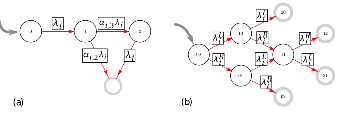
Figure S1. Two graphical representations of the WTD (S22). The waiting time is equal to the adsorption time of a random walker from the leftmost site to any of the grey sites.
WTD (S21). Equation (38) of the main text follows straightforwardly. A comparison with (S20) shows that it corresponds to the case with three stages (i.e., k = 3),
p0=p1= 0, andp2=αRi,2+αi,L2. Hence, the jump fromxi toxj can be modelled as a process of three stages, in each of which the system is trapped for an exponentially distributed time with rate λi. At time zero, with probability 1, the system enters the first stage and waits there. Then, again with probability 1, it enters a second identical stage. After leaving the second stage, the escape occurs immediately with probabilityp2, or the system enters the third and last phase with probability 1−p2.
Hence the WTD is the time to absorption of the Markov process with the transition graph of figure S1(a), given that we start at state 0. Recalling the notion of trigger, it is possible to build an alternative but equivalent absorbing Markov process with the same time to absorption. We think of each of the two Gamma triggers (R or L) as a device with two exponential stages (with rateλRi or λLi). The escape occurs when either of the two triggers leaves the last stage. The transition graph of the associated Markov processes is shown in figure S1(b).
/
/
/
/ (
) )
) (
(
)
(
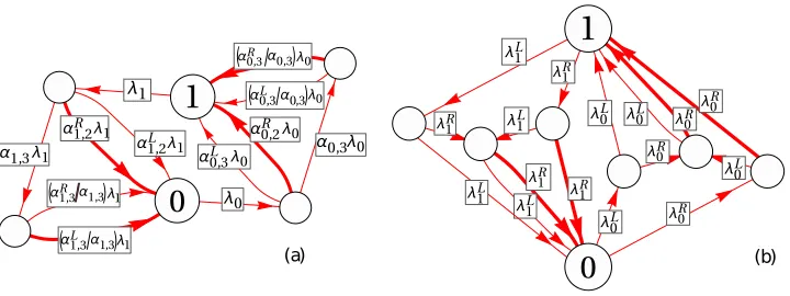
[image:24.612.108.468.101.236.2](a) (b)
Figure S2. Graphical representations of the non-DTI ion-channel model with hidden states. The bonds corresponding to biased rates are drawn in thick lines. The modified generators associated with these two models have the same leading eigenvalue. (a) and (b) correspond to the WTD representations of figure S1.
References
[S1] E. W. Montroll and G. H. Weiss. Random walks on lattices. II. J. Math. Phys., 6(2):167, 1965. [S2] J. W. Haus and K. W. Kehr. Diffusion in regular and disordered lattices. Phys. Rep.,
150(5-6):263–406, 1987.
[S3] M. Esposito and K. Lindenberg. Continuous-time random walk for open systems: fluctuation theorems and counting statistics. Phys. Rev. E, 77(5):051119, 2008.
[S4] D. R. Cox. Renewal Theory. London UK, Methuen & Co., 1967.
[S5] M. F. Shlesinger Asymptotic solutions of continuous-time random walks. J. Stat. Phys., 10(5):421–434, 1974.
[S6] P. S. Efraimidis and P. G. Spirakis. Weighted random sampling with a reservoir. Inf. Process. Lett., 97(5):181–185, 2006.
[S7] C. Giardin`a, J. Kurchan, and L. Peliti. Direct evaluation of large-deviation functions. Phys. Rev. Lett., 96(12):120603, 2006.
[S8] W. J. Stewart. Probability, Markov Chains, Queues, and Simulation: The Mathematical Basis of Performance Modeling. Princeton NJ, Princeton University Press, 2009.

![Figure 2.SCGF of current in ion channel. (a) DTI model with (k0, λ0, k1, λ1) =(0.1, 0.01, 1, 1) and (px1,x0,1, px0,x1,0, px0,x1,−1, px1,x0,0) = (0.5, 0.6, 0.4, 0.5); thecloning result is consistent with the solution given in [38]](https://thumb-us.123doks.com/thumbv2/123dok_us/9467704.453185/11.612.101.468.100.236/figure-current-channel-model-thecloning-result-consistent-solution.webp)
![Figure 3.(a) Cloning evaluation of the SCGF for the non-Markovian TASEP,(the thermodynamic integration of [11]](https://thumb-us.123doks.com/thumbv2/123dok_us/9467704.453185/13.612.103.463.104.234/figure-cloning-evaluation-scgf-markovian-tasep-thermodynamic-integration.webp)