Double obstacle phase field approach to an inverse problem for a discontinuous diffusion coefficient

warwick.ac.uk/lib-publications

Original citation:

Deckelnick, Klaus, Elliott, Charles M. and Styles, Vanessa. (2016) Double obstacle phase field approach to an inverse problem for a discontinuous diffusion coefficient. Inverse Problems, 32 (4). 045008.

Permanent WRAP URL:

http://wrap.warwick.ac.uk/76384

Copyright and reuse:

The Warwick Research Archive Portal (WRAP) makes this work by researchers of the University of Warwick available open access under the following conditions. Copyright © and all moral rights to the version of the paper presented here belong to the individual author(s) and/or other copyright owners. To the extent reasonable and practicable the material made available in WRAP has been checked for eligibility before being made available.

Copies of full items can be used for personal research or study, educational, or not-for-profit purposes without prior permission or charge. Provided that the authors, title and full

bibliographic details are credited, a hyperlink and/or URL is given for the original metadata page and the content is not changed in any way.

Publisher’s statement:

"This is an author-created, un-copyedited version of an article accepted for

publication/published in [insert name of journal]. IOP Publishing Ltd is not responsible for any errors or omissions in this version of the manuscript or any version derived from it. The Version of Record is available online at http://dx.doi.org/10.1088/0266-5611/32/4/045008

A note on versions:

The version presented here may differ from the published version or, version of record, if you wish to cite this item you are advised to consult the publisher’s version. Please see the ‘permanent WRAP URL’ above for details on accessing the published version and note that access may require a subscription.

Double obstacle phase field approach to an inverse problem

for a discontinuous diffusion coefficient

Klaus Deckelnick∗, Charles M. Elliott†and Vanessa Styles‡

Abstract

We propose a double obstacle phase field approach to the recovery of piece-wise constant diffusion coefficients for elliptic partial differential equations. The approach to this inverse problem is that of optimal control in which we have a quadratic fidelity term to which we add a perimeter regularisation weighted by a parameterσ. This yields a functional which is optimised over a set of diffusion coefficients subject to a state equation which is the underlying elliptic PDE. In order to derive a problem which is amenable to computation the perimeter functional is relaxed using a gradient energy functional together with an obstacle potential in which there is an interface parameter

. This phase field approach is justified by proving Γ−convergence to the functional with perimeter regularisation as→0. The computational approach is based on a finite element approximation. This discretisation is shown to converge in an appropriate way to the solution of the phase field problem. We derive an iterative method which is shown to yield an energy decreasing sequence converging to a discrete critical point. The efficacy of the approach is illustrated with numerical experiments.

1

Introduction

Many applications lead to mathematical models involving elliptic equations with piece-wise constant discontinuous coefficients. Frequently the interfaces across which the coefficients jump are completely unknown. A common approach for the identification of these coef-ficients is to make observations of the field variables solving the equations and use these values in an attempt to determine the coefficients by formulating an inverse problem for the coefficients. This is generally ill posed and in applications it is usual to use a fidelity to the observations functional together with a regularisation of the coefficients. In this paper we use a regularisation of the coefficients by employing the perimeter of the jump sets of the coefficients.

∗

Institut f¨ur Analysis und Numerik, Otto-von-Guericke-Universit¨at Magdeburg, Universit¨atsplatz 2, 39106 Magdeburg, Germany.

†

Mathematics Institute, University of Warwick, Coventry CV4 7AL, UK.

‡

Department of Mathematics, University of Sussex, Brighton BN1 9RF, UK.

1.1 Model problem

To fix ideas we consider the following model elliptic problem:

− ∇ · a∇y = 0 in Ω (1.1)

a∂y

∂ν = g on∂Ω, (1.2)

where Ω is a bounded domain inRd(d= 2,3), g is given boundary data with zero mean

Z

∂Ω

g= 0 (1.3)

and a is an isotropic diffusion (conductivity) coefficient. We suppose that the diffusion coefficient takes one of the r positive values a1, . . . , ar. Our interest is in modelling a

geometrical inverse problem concerning the determination of the regions in which the ma-terial diffusion coefficient takes these values. Our problem then is to determine the sets Ei={x∈Ω|a(x) =ai}given observations of the solution yof the elliptic boundary value

problem (1.1), (1.2). In the case of r = 2, under constraints on the nature of the domains and boundary conditions, uniqueness and stability results have been proved in [7, 2]. In this context see also [28].

A standard approach is to minimise a fidelity functional Jf id(E) :=||yE−yobs||2O

over an appropriate class of partitions E = (Ei)ri=1 of Ω, where yE denotes the solution of

the state or forward equation (1.1), (1.2) with diffusion coefficient a(x) = ai, x ∈ Ei, i =

1, . . . , r. Furthermore, O is an appropriate space of observations and yobs ∈ O is given.

In general this problem is ill-posed and is typically regularised by adding a Tikhonov regularisation functional. A numerical approach without regularisation is proposed in [28, 32].

1.2 Geometric regularisation

In this setting it has been considered appropriate to use perimeter regularisation, [34, 31]

Jreg(E) = ˆσ r

X

i=1

Hd−1(∂Ei∩Ω), E = (Ei)ri=1,

where the regularisation parameter ˆσ is positive. Minimisers of J(E) :=Jf id(E) +Jreg(E)

are then typically sought in the set of Caccioppoli partitions intor components, i.e. par-titions E = (Ei)ri=1 of Ω with Hd(Ei ∩Ej) = 0, i 6= j, Hd Ω\Sri=1Ei

= 0 for which ui := χEi belongs to BV(Ω), i = 1, . . . , r. Thus, a Caccioppoli partition corresponds to a

function u = (u1, . . . , ur) ∈ BV(Ω,{e1, . . . , er}), where e1, . . . , er are the unit vectors in

Rr. We can then write the regularisation functional in terms of u as follows:

Jreg(u) = ˆσ r

X

i=1

Z

Ω

Here, R_Ω|Dui| is the total variation of the vector–valued Radon measure Dui. Before we

rewrite the fidelity term let us introduce the Gibbs simplex

Σ :={y∈_Rr_|y

i ≥0, i= 1, . . . , r, r

X

i=1

yi= 1}

and observe thate1, . . . , er are the corners of Σ. Consider the set

X:={u: Ω→_Rr|u is measurable and u(x)∈Σ a.e. in Ω}

endowed with the L1–norm and define foru∈X

a(u) :=

r

X

i=1

aiui (1.4)

and byS(u) the solution of (1.1), (1.2) with diffusion coefficient a(u).

We set ˆσ = π₈σ for later convenience. The constant π/8 arises from the form of the phase field relaxation used in (1.5), see (2.7).

Problem (PGR) is then to seek minimizers of the functionalJ :X→_R∪ {∞}given by

J(u) :=

      

1

2||S(u)−yobs||

2

O+σ

π 8

r

X

i=1

Z

Ω

|Dui| , ifu∈BV(Ω,{e1, . . . , er})∩X;

∞ , otherwise.

In this problem the fidelity term is non-convex because of the nonlinearity of the state solution operator S(·) with respect to the coefficient a(u). Also a feature of this natural geometric regularisation approach is that the regularisation functional is non-convex. This is reflected in the fact that u only takes one of the values e1, . . . , er which leads to a

non–convex constraint.

1.3 Double obstacle phase field approach

We shall consider a suitable phase field approximation of the above regularisation which involves gradient energies and functions that map into the Gibbs simplex. In this approxi-mation we relax the non-convex constraintu(x)∈ {e1, . . . , er}by introducing the set

K :={u∈H1(Ω,Rr)|u(x)∈Σ a.e. in Ω}

and approximateJ by the sequence of functionals J:X →R∪ {∞}, >0 with

J(u) :=

    

1

2||S(u)−yobs||

2

O+σ

Z

Ω

ε 2|Du|

2₊ 1

2ε(1− |u|

2₎

dx , ifu∈ K;

∞ , otherwise.

(1.5)

Here,R_Ω|Du|2_dx=Pr

i=1

R

Ω|∇ui|

2_{dxand foru∈ Kwe have}R

Ω(1− |u|

2_{) =}Pr

i=1

R

Ωui(1−

ui). Problem (PDO) is then to seek minimisers ofJε. We refer to this approach as a double

obstacle phase field model because of the constraints 0≤ui≤1 on the components of the

separating two sets on which the diffusion coefficient is constant. The Cahn–Hilliard type energy

Z

Ω

ε 2|∇u|

2₊ 1

2ε(u−u

2₎

dx

is well established as an approximation of the perimeter functional, see e.g. [12, 11, 6]. Note that the regularisation remains non-convex through the quadratic Cahn-Hilliard functional even though the constraint set is convex. Let us remark that such a phase field model has recently been used in a binary recovery problem, see [15].

Note that we view (PGO) as having just one regularisation parameterσ. Theεparameter in (PGO) may be viewed as a way of providing an approximation of (PGR) which is computationally accessible.

1.4 Other approaches

There have been attempts to solve the recovery problem without regularisation of the inter-faces across which the diffusion coefficients jump. Formally one can write down variations of the fidelity functional with respect to variations of the interfaces. For example see [28]. In particular the interfaces can be associated with particular level sets of level set functions which have to be determined. We refer to [36, 32, 24, 16] for numerical implementations. The use of level set descriptions of the interfaces in the context of perimeter regularisations is described in [3, 26, 27]. Related to this is the use of total variation of a regularised Heavi-side function with argument being a level set function, [22, 40]. In [19] the authors conHeavi-sider the distributed control of linear elliptic systems in which the control variable should only take on a finite number of values. To this purpose they introduce a combination ofL2 and L0–type penalties whose Fenchel conjugates allow the derivation of a primal–dual opti-mality system with a unique solution. A suitable adaption of this approach could be an alternative way to attack the inverse problem considered in the present paper.

In the different context of image segmentation parametric description of curves have been used in conjunction with perimeter regularisation, [8, 39].

On the other hand [17, 38, 35] use total variation regularisation and relax the constraints that the indicator functions take just two values.

1.5 Applications

Our model problem is an example of the identification of a coefficient in an elliptic equation. This problem arises in many applications. For example, a fundamental issue in the use of mathematical models of flow in porous media is that the geological features which determine the permeability are unknown. In geology a facies is a body of rock with specific characteristics. In our model problemy is the pressure or hydraulic head associated with a fluid (for example, oil or water) occupying the reservoir or acquifer Ω and a is the permeability of the rock. We assume that the permeability is isotropic and is piece-wise constant. The domainsEi={x∈Ω|a(x) =ai}, i= 1,2, ..., rmodel the decomposition of

Such problems also arise in imaging. For example, electric impedance tomography, [18, 24, 13], is the determination of the conductivity distribution in the interior of a domain using observations of current and potential. Hereyis the electric potential andais a conductivity which takes different values in unknown interior domains. In medical imaging the shape and size of interior domains may be inferred from the variation of the conductivity.

1.6 Outline and contributions of the paper

• In Section 2 we introduce the functionals J and prove that they Γ–converge to J.

Furthermore, we show that J has a minimum and derive a necessary first order

condition. This establishes that problems (PGR) and (PDO) have solutions.

• The optimisation problem in Section 2 is infinite-dimensional. In order to carry out numerical calculations we employ a finite element spatial discretisation. This is de-rived in Section 3 and we prove convergence results for absolute minimizers and crit-ical points as the mesh size tends to zero. This establishes that the inverse problems (PGR) and (PDO) can be approximated by something computable.

• Section 4 is devoted to formulating an iterative scheme for finding critical points of the functional associated with the discrete optimisation problem. The method is based on a semi-implicit time discretisation of a parabolic variational inequality which is a gradient flow for the energy. In this finite dimensional setting we prove a global convergence result for the iteration.

• Finally in Section 5 we illustrate the applicability of the method with some numerical examples.

2

Problem formulation

2.1 State equation

Let Ω⊂Rdbe a bounded domain with a Lipschitz boundary. We suppose thatg∈L2(∂Ω)

satisfying (1.3) andyobs ∈ Oare given functions. Here, O,(·,·)O

is a Hilbert space with the property that H1(Ω) is compactly embedded in O. Furthermore we assume that the following Poincar´e inequality

||η− MO(η)|| ≤Cp||∇η||, η∈H1(Ω) (2.1)

holds, where|| · || denotes theL2(Ω) norm and MO(η) denotes the mean value of η with

MO(η) := (η,1)O/||1||2O, η∈ O.

Typical examples are O = L2(Ω) or L2(∂Ω) representing either bulk measurements or boundary observations of the solution of the state equation.

For a given u ∈ X we denote by y = S(u) ∈ H1(Ω) the unique weak solution of the Neumann problem

− ∇ ·(a(u)∇y) = 0 in Ω (2.2)

a(u)∂y

withMO(y) =MO(yobs) in the sense that

Z

Ω

a(u)∇y· ∇ηdx=

Z

∂Ω

gηdo ∀η∈H1(Ω). (2.4)

Here,a(u) is given by (1.4), where we note that

amin ≤a(u)≤amax a.e. in Ω, uniformly inu∈X, (2.5)

where amin := min(a1, . . . , ar), amax := max(a1, . . . , ar). Observe that S is a nonlinear

operator because of the bilinear relation betweena(u) andy in (2.4). Using (2.1) together with the fact thatMO(y) =MO(yobs) we infer that the solutiony =S(u) satisfies

kyk ≤ ky− MO(y)k+|Ω| 1

2|M_O(y_obs)| ≤C_pk∇yk+ |Ω| 1 2

||1||O

kyobskO.

If we combine this estimate with the choice η = y in (2.4) and use (2.5) as well as the continuous embeddingH1_(Ω),→L2_{(∂Ω) we deduce that}

kS(u)k_H1_(Ω) ≤c(a_min,Ω) kgk_L2_(∂Ω)+ky_obsk_O uniformly in u∈X. (2.6)

We see that the problem of observing y givenu is well formulated because

S :X→ O is continuous

which is a consequence of the following lemma.

Lemma 2.1. S :X→H1(Ω) is continuous.

Proof. Letu ∈X and (uk)k∈N a sequence in X withuk →u inL1(Ω,Rr), k → ∞. Since

0 ≤ uk,i ≤ 1, i = 1, . . . , r we may assume by passing to a subsequence if necessary that

uk → u in L2(Ω,Rr) and a.e. in Ω. Abbreviating y = S(u), yk = S(uk) we have for

η∈H1(Ω)

Z

Ω

a(uk)∇(yk−y)· ∇ηdx=

Z

Ω

(a(u)−a(uk))∇y· ∇ηdx.

Choosingη=yk−y we deduce with the help of (2.5) and (1.4)

amink∇(yk−y)k ≤amax

Z

Ω

|uk−u|2|∇y|2dx

1

2

→0, k→ ∞

by the dominated convergence theorem because

|uk−u|2|∇y|2→0 a.e. in Ω, |uk−u|2|∇y|2 ≤r|∇y|2 a.e in Ω and |∇y|2 ∈L1(Ω).

Since MO(yk−y) = 0 we deduce with the help of (2.1) that S(uk) =yk → y =S(u) in

2.2 Γ–convergence and existence of minimizers

The use ofJ in the minimization ofJ is justified by the following Γ–convergence result.

Theorem 2.2. The functionals J Γ–converge to J in X.

Proof.Let us write J(u) =G(u) +σF(u), where G(u) = 1₂||S(u)−yobs||2O is continuous

as a consequence of Lemma 2.1 and the embedding of H1(Ω) into O. In Theorem 6.1 in the Appendix we show that

F

Γ

→F, where F(u) =

      

π 8

r

X

i=1

Z

Ω

|Dui| , ifu∈BV(Ω,{e1, . . . , er})∩X;

∞ , otherwise.

(2.7)

Using Remark 1.7 in [14] we infer thatJ

Γ

→G+σF =J.

Theorem 2.3. The minimization problem minv∈XJ(v) has a solution u ∈ K.

Proof. Let (uk)k∈_N ⊂ Kbe a minimizing sequence, J(uk) & infv∈XJ(v). Since (uk)k∈_N

is bounded in H1_(Ω,

Rr) there exists a subsequence, again denoted by (uk)k∈N, and u ∈

H1(Ω,Rr) such that

uk*u inH1(Ω,Rr), uk→u inL2(Ω,Rr) and a.e. in Ω.

In particular, u ∈ K. Lemma 2.1 implies that S(uk)→ S(u) in O which combined with

the weak lower semicontinuity of theH1-seminorm shows thatu is a minimum of J.

Corollary 2.4. Let (u)>0be a sequence of minimizers ofJ. Then there exists a sequence

k →0, k→ ∞ andu∈BV(Ω;{e1, . . . , er})∩X such thatuk →u in L

1_(Ω,

Rr) andu is

a minimum ofJ.

Proof. By Corollary 6.2 in the Appendix there exists a sequence k → 0, k → ∞ and

u ∈ BV(Ω;{e1, . . . , er})∩X such that uk → u in L

1_(Ω,

Rr). It is well–known that the

Γ–convergence ofJk toJ implies thatu is a minimum ofJ.

2.3 Necessary first order condition for the phase field recovery

In order to derive the necessary first order conditions for a minimum ofJεwe considerK as

a subset ofL∞(Ω,Rr). Similarly as in [9], Section 3, one can prove that the solution operator

S : L∞(Ω,Rr) ⊃ K → H1(Ω) is Fr´echet differentiable with ˜y = S0(u)w,w ∈ L∞(Ω,Rr)

being given as the solution of

Z

Ω

a(u)∇y˜· ∇ηdx=−

Z

Ω

a(w)∇S(u)· ∇ηdx ∀η∈H1(Ω) (2.8)

withMO(˜y) = 0. As a result, Jε is Fr´echet differentiable on K ⊂L∞(Ω,Rr)∩H1(Ω,Rr)

with

J_ε0(u)w= S(u)−yobs, S0(u)w

O+σ

Z

Ω

εDu·Dw−1

εu·w

for w ∈ L∞(Ω,Rr)∩H1(Ω,Rr). In order to avoid the evaluation of S0(u)w in (2.9) we

work as usual with a dual problem: Findp∈H1(Ω) such that MO(p) = 0 and

Z

Ω

a(u)∇p· ∇ηdx= S(u)−yobs, η

O ∀η ∈H

1_{(Ω), (2.10)}

where we note that the solvability condition S(u)−yobs,1

O = 0 is satisfied. As a result

we obtain from (2.9), (2.10) and (2.8)

J_ε0(u)w =

Z

Ω

a(u)∇p· ∇[S0(u)w]dx+σ

Z

Ω

εDu·Dw−1

εu·w

dx

= −

Z

Ω

a(w)∇S(u)· ∇pdx+σ

Z

Ω

εDu·Dw−1

εu·w

dx.

At a minimumuofJ we haveJε0(u)(v−u)≥0 for allv∈ K. Sincea(v−u) =a(v)−a(u)

we therefore define:

Definition 2.5. (Phase field critical point) Find u∈ K such that for allv∈ K

σ

Z

Ω

εDu·D(v−u)−1

εu·(v−u)

dx−

Z

Ω

(a(v)−a(u))∇S(u)· ∇pdx≥0. (2.11)

Remark 2.6. A natural strategy to construct solutions of (2.11) and hence to find can-didates for at least a local minimum of Jε is to consider the following parabolic obstacle

problem: Findu(·, t)∈ K, t≥0 such thatu(·,0) =u0 and

(ut,v−u) +σ

Z

Ω

εDu·D(v−u)−1

εu·(v−u)

dx−

Z

Ω

(a(v)−a(u))∇S(u)· ∇pdx≥0

for all v ∈ K and all t > 0. Here, p is the solution of (2.10) for u(·, t) and u0 ∈ K is a

suitably chosen initial function.

Inserting v=u(·, t−∆t) into the above relation, dividing by ∆t and sending ∆t→0 we formally find that

kutk2+J0(u)ut≤0,

so that d

dtJ(u(·, t)) ≤ 0 and the value of the objective funtional decreases during the evolution. If limt→∞u(·, t) =:u∞ exists, we expect u∞ to be a solution of (2.11).

3

Finite element approximation

In what follows we assume that Ω is a polygonal (d=2) or polyhedral (d=3) domain. Let us denote by (Th)0<h≤h0 a regular triangulation of Ω and set

Vh ={χ∈C0( ¯Ω)|χ|T ∈P1(T) for all T ∈ Th} ⊂H1(Ω)

as well as

Using the construction of the Cl´ement interpolation operator ([20]) it is not difficult to see that for everyu∈ K there exists a sequence (ˆuh)0<h≤h0 with ˆuh∈ Kh such that

ˆ

uh →u inH1(Ω,Rr) as h→0. (3.1)

Furthermore, let (y_obsh )0<h≤h0 be a sequence of functions y

h

obs ∈ O such that

y_obsh →yobs inO ash→0. (3.2)

Foruh∈ Kh we denote byyh =Sh(uh)∈Vh the solution of

Z

Ω

a(uh)∇yh· ∇χdx=

Z

∂Ω

ghχdo ∀χ∈Vh (3.3)

withMO(yh) =MO(y_obsh ). Heregh :∂Ω→Ris a piecewise linear, continuous

approxima-tion tog satisfying

Z

∂Ω

ghdo= 0 and gh→g inL2(∂Ω) as h→0. (3.4)

In the same way as in (2.6) one can prove that

kSh(uh)kH1 ≤c kg_hk_L2_(∂Ω)+ky_obsh k_O

≤c uniformly inuh∈ Kh, (3.5)

where the constantc is independent of hin view of (3.2) and (3.4).

Lemma 3.1. Let (hk)k∈N be a sequence with limk→∞hk= 0 and uhk ∈ Khk withuhk →u

in L1(Ω,Rr). Then Shk(uhk)→S(u) in H

1_{(Ω), k→ ∞.}

Proof.Letuk=uhk, yk =Shk(uk) andy=S(u). By passing to a subsequence if necessary

we may assume in addition that uk →u a.e. in Ω. Choose a sequence ˆyk ∈Vhk such that

ˆ

yk→y inH1(Ω). Using (2.1) we deduce

kyk−yˆkkH1 ≤ ky_k−yˆ_k− M_O(y_k−yˆ_k)k+|Ω| 1

2|M_O(yhk

obs−yˆk)|+k∇(yk−yˆk)k ≤ ck∇(yk−yˆk)k+|Ω|

1

2 |M_O(yhk

obs−yobs)|+|MO(y−yˆk)|

≤ ck∇(yk−yˆk)k+c(ky_obshk −yobskO+ky−yˆkkH1). (3.6)

In order to estimate the first term we write

Z

Ω

a(uk)∇(yk−yˆk)· ∇χdx

=

Z

Ω

a(uk)∇(y−yˆk)· ∇χdx+

Z

Ω

a(u)−a(uk)

∇y· ∇χdx+

Z

∂Ω

(ghk−g)χdo

for allχ∈Vhk. If we letχ=yk−yˆk and take into account (3.6) we obtain

kyk−yˆkkH1 ≤ cky−yˆ_kk_H1 +c

Z

Ω

|uk−u|2|∇y|2dx

1

2

+c kghk−gkL2(∂Ω)+ky

hk

obs−yobskO

by (3.4) and (3.2). Here, the second integral is shown to converge to zero in the same way as in the proof of Lemma 2.1. In conclusion, Shk(uhk) = (yk−yˆk) + ˆyk → y = S(u) in

H1(Ω) and by a standard argument the whole sequence converges. UsingSh we define the following approximation J,h:Kh →R ofJ:

J,h(uh) :=

1

2||Sh(uh)−y

h

obs||2O+σ

Z

Ω

ε 2|Duh|

2₊ 1

2ε(1− |uh|

2₎

dx. (3.7)

Theorem 3.2. There exists uh ∈ Kh such that J,h(uh) = minvh∈KhJ,h(vh). Every

sequence (uhk)k∈N with limk→∞hk = 0 has a subsequence that converges strongly in

H1_(Ω,

Rr) and a.e. in Ωto a minimum of J.

Proof.SinceXhis finite-dimensional, the existence of a minimum ofJ,his straightforward.

Next, letuk∈ Khk be a sequence with limk→∞hk= 0 andJ,hk(uk) = minvh∈K_hkJ,hk(vh).

Since (uk)k∈N is bounded in H1(Ω,Rr), there exists a subsequence, again denoted by

(uk)k∈N, and u∈ K such that

uk*u inH1(Ω,Rr), uk→u inL1(Ω,Rr) and a.e. in Ω. (3.8)

Furthermore, Lemma 3.1 implies that

Shk(uk)→S(u) inH

1_{(Ω). (3.9)}

We claim thatu is a minimum ofJ. To see this, let v ∈ K be arbitrary and ˆvk ∈ Khk a

sequence with ˆvk →vinH1(Ω,Rr), see (3.1). Since J,hk(uk)≤J,hk(ˆvk) we deduce from

(3.8), (3.9) and again Lemma 3.1 that

J(u)≤lim inf

k→∞ J,hk(uk)≤lim sup_k→∞ J,hk(uk)≤klim→∞J,hk(ˆvk) =J(v),

so that J(u) = minv∈XJ(v). Furthermore, by repeating the above argument with a

sequence ˆuk∈ Khk such that ˆuk →u inH

1_(Ω,

Rr) we infer in addition that

lim

k→∞J,hk(uk) =J(u). (3.10)

We use this relation to show thatkDukk2→ kDuk2. Namely, let us write

σ 2

Z

Ω

|Duk|2dx = J,hk(uk)−

σ 2

Z

Ω

(1− |uk|2)dx−

1

2kShk(uk)−y

hk

obsk

2

O

→ J(u)−

σ 2

Z

Ω

(1− |u|2)dx−1

2kS(u)−yobsk

2

O=

σ 2

Z

Ω

|Du|2dx

in view of (3.10), (3.8), (3.9) and (3.2). Hence uk → u in H1(Ω,Rr) and the theorem is

proved.

In practice, rather than trying to locate a global minimum ofJ,h one looks for admissible

pointsuh that satisfy the necessary first order condition

A calculation analogous to (2.11) leads us to the following variational inequality:

σ

Z

Ω

εDuh·D(vh−uh)−

1

εuh·(vh−uh)

dx−

Z

Ω

(a(vh)−a(uh))∇yh· ∇phdx≥0 (3.12)

for all vh ∈ Kh, where yh =Sh(uh) and ph ∈Vh withMO(ph) = 0 is the solution of the

discrete adjoint problem:

Z

Ω

a(uh)∇ph· ∇χdx= (yh−yhobs, χ)O ∀χ∈Vh. (3.13)

Theorem 3.3. Let (uhk)k∈N be a sequence of solutions of (3.12) with limk→∞hk = 0.

Then there exists a subsequence that converges strongly in H1(Ω,Rr) and a.e. in Ω to a

solution u of (2.11).

Proof. Let us abbreviate uk =uhk, yk =Shk(uk) and denote by pk ∈ Vhk the solution of

(3.13) withuh =uk andyh=yk. Using (3.5) and testing (3.13) withχ=pk we infer that kykkH1+kp_kk_H1 ≤c uniformly ink∈_N.

Next, inserting vh≡ 1_rPr_j=1ej into (3.12) we deduce

σε

Z

Ω

|Duk|2dx ≤

σ ε

Z

Ω

|uk|2dx+

Z

Ω

(a(uk)−

1 r

r

X

i=1

ai)∇yk· ∇pkdx

≤ σr

ε |Ω|+ck∇ykk k∇pkk ≤c.

Hence, there exists a subsequence, again denoted by (uk)k∈N, and u∈ K such that

uk*u inH1(Ω,Rr), uk→u inL1(Ω,Rr) and a.e. in Ω. (3.14)

Lemma 3.1 implies that

yk=Shk(uk)→S(u) =:y inH

1_{(Ω). (3.15)}

Let p∈H1(Ω),MO(p) = 0 be the solution of (2.10). Choose ˆpk ∈Vhk with MO(ˆpk) = 0

such that ˆpk →p inH1(Ω) and write

Z

Ω

a(uk)∇(pk−pˆk)· ∇χdx=

Z

Ω

a(uk)∇(p−pˆk)· ∇χdx

+

Z

Ω

a(u)−a(uk)

∇p· ∇χdx+ (yk−y, χ)O−(y_obshk −yobs, χ)O

for allχ∈Vhk. By choosingχ=pk−pˆk and using (2.1), (3.15) and (3.2) we deduce

kpk−pˆkkH1 ≤ckpˆ_k−pk_H1+c

Z

Ω

|uk−u|2|∇p|2dx

1

2

+c kyk−ykO+kyh_obsk −yobskO

→0

which implies that pk→p inH1(Ω).

Let us next show that u satisfies (2.11). Given v ∈ K there exists a sequence ˆvk ∈ Khk

such that ˆvk→v inH1(Ω,Rr) and a.e. in Ω. Then we have from (3.12)

σ

Z

Ω

εDuk·D(ˆvk−uk)−

1

εuk·(ˆvk−uk)

dx−

Z

Ω

In order to examine the second term we write

Z

Ω

(a(ˆvk)−a(uk))∇yk· ∇pkdx−

Z

Ω

(a(v)−a(u))∇y· ∇pdx (3.17)

=

Z

Ω

(a(ˆvk)−a(uk))[∇(yk−y)· ∇pk+∇y· ∇(pk−p)]dx

+

Z

Ω

(a(ˆvk)−a(v))−(a(uk)−a(u))

∇y· ∇pdx→0, k→ ∞

sinceyk → y, pk → p in H1(Ω) where we used again the dominated convergence theorem

for the second integral. By passing to the limit in (3.16) and observing thatR_Ω|Du|2_dx≤

lim infk→∞R_Ω|Duk|2dxwe infer thatu satisfies (2.11).

Let us finally show that uk → u in H1(Ω,Rr). Choose a sequence ˆuk ∈ Khk such that

ˆ

uk→u inH1(Ω,Rr). Inserting vhk = ˆuk into (3.12) we obtain

σ

Z

Ω

|Duk|2dx≤σ

Z

Ω

Duk·Duˆkdx−

σ

Z

Ω

uk·(ˆuk−uk)dx−

Z

Ω

a(ˆuk)−a(uk)

∇yk·∇pkdx

so that (3.14) and (3.17) with ˆvk= ˆuk imply that

lim sup

k→∞

Z

Ω

|Duk|2dx≤

Z

Ω

|Du|2_dx.

HenceR_Ω|Duk|2dx→

R

Ω|Du|2dx, so that Duk→Du inL2.

4

An iterative scheme

4.1 Iterative method

Let us consider the following iteration, which can be seen as a time discretization of the parabolic obstacle problem introduced in Remark 2.6. Given un_h ∈ Kh let un_h+1 ∈ Kh be

the solution of the problem

Z

Ω

(un_h+1−un_h)·(vh−un_h+1)dx−τn

Z

Ω

(a(vh)−a(u_hn+1))∇ynh· ∇pnhdx (4.1)

+τnσ

Z

Ω

εDun_h+1·D(vh−un_h+1)−

1 εu

n

h·(vh−un_h+1)

dx≥0 ∀vh ∈ Kh,

whereτn>0, ynh =Sh(unh) and pnh ∈Vh solves the discrete dual problem

Z

Ω

a(un_h)∇p_hn· ∇χdx= (yn_h−y_obsh , χ)O ∀χ∈Vh withMO(pnh) = 0. (4.2)

Note thatun_h+1 is the unique solution of the convex minimization problem

min

vh∈Kh

1

2kvh−u

n hk2−τn

Z

Ω

a(vh)∇yhn· ∇pnhdx+τnσ

Z

Ω

2|Dvh|

2_dx− 1

u

n h·vh

4.2 Convergence of the iterative method

The following result shows that the objective functional decreases in the iteration provided the time stepsτn satisfy a suitable condition. In order to formulate it we define

ˆ a:=

r

X

i=1

a2_i

1

2_{, ˆc:= inf}

nR

Ω|∇η| 2_dx

kηk2

O

|η∈H1(Ω)\ {0},MO(η) = 0

o

. (4.3)

Note that ˆc≥C_p2 >0 in view of (2.1).

Lemma 4.1. The sequence (un_h)n∈N0 satisfies

kun_h+1−un_hk2+J,h(u_hn+1)≤J,h(unh), n∈N0,

provided that

τn≤

1 + ˆa

2

amin

k∇yn_hk_L∞k∇pn

hkL∞+ ˆa

2

a2_min 1 2ˆck∇y

n hk2L∞

−1

, n∈_N0. (4.4)

Proof.Inserting χ=un

h into (4.1) we obtain after some calculations

1 τn

kun_h+1−un_hk2₊σ

2 kD(u

n+1

h −u n h)k2+

σ 2ku

n+1

h −u n hk2

+σ

Z

Ω

2|Du

n+1

h |

2₊ 1

2(1− |u

n+1

h |

2₎

dx−σ

Z

Ω

2|Du

n h|2+

1

2(1− |u

n h|2)

dx

≤

Z

Ω

a(un_h+1)∇yn_h· ∇pn_hdx−

Z

Ω

a(un_h)∇yn_h· ∇pn_hdx≡:I+II. (4.5)

Using (3.3) for yn_h and y_hn+1 with test function pn_h as well as (3.13) we may rewrite II as follows:

II = −

Z

Ω

a(un_h+1)∇y_hn+1· ∇pn_hdx (4.6)

= −

Z

Ω

a(un_h+1)∇y_hn+1· ∇pn_h+1dx+

Z

Ω

a(un_h+1)∇yn_h+1· ∇(pn_h+1−pn_h)dx

= −(y_hn+1−y_obsh , y_hn+1)O+

Z

Ω

a(un_h+1)∇yn_h+1· ∇(p_hn+1−pn_h)dx≡II1+II2.

Using again (3.13) we may write

II1 = −

1 2||y

n+1

h −y h obs||2O+

1 2||y

n

h −yhobs||2O−

1 2||y

n+1

h −y n

h||2O−(ynh+1−y h

obs, ynh)O

= −1

2||y

n+1

h −y h obs||2O+

1 2||y

n

h −yhobs||2O−

1 2||y

n+1

h −y n h||2O

−

Z

Ω

a(un_h+1)∇yn_h· ∇pn_h+1dx,

while

II2 =

Z

Ω

Inserting the above identities into (4.6) and combining it with (4.5) we obtain 1 τn + σ 2

kun_h+1−un_hk2+σ 2 kD(u

n+1

h −u n h)k2+

1 2||y

n+1

h −y n

h||2O+J,h(unh+1)

≤ J,h(unh) +

Z

Ω

a(un_h)−a(un_h+1)∇y_hn· ∇(pn_h+1−pn_h)dx

≤ J,h(unh) + ˆak∇yhnkL∞kun+1 h −u

n

hk k∇(pnh+1−p n

h)k. (4.7)

It remains to estimatek∇(pn_h+1−pn_h)k. To begin, note that

Z

Ω

a(un_h+1)∇(p_hn+1−pn_h)· ∇χdx=

Z

Ω

(a(un_h)−a(un_h+1))∇pn_h· ∇χdx+ (yn_h+1−yn_h, χ)O

for allχ∈Vh. Inserting χ=pnh+1−pnh we deduce that

amink∇(pn_h+1−pnh)k2 ≤ ˆak∇pn_hk_L∞kun+1

h −u n

hk k∇(pnh+1−p n

h)k+kyhn+1−y n

hkOkpn_h+1−pnhkO,

which implies in view of (4.3)

k∇(pn_h+1−pn_h)k ≤ ˆa

amin

k∇pn_hk_L∞kun+1 h −u

n hk+

1 √ ˆ c 1 amin

ky_hn+1−y_hnkO.

Inserting the above bounds into (4.7) and using (4.4) we infer 1

τn

kun_h+1−un_hk2+σ 2 kD(u

n+1

h −u n h)k2+

1 2||y

n+1

h −y n

h||2O+J,h(uhn+1)−J,h(unh)

≤ ˆa

2

amin

k∇y_hnk_L∞k∇pn_hk_L∞kun+1 h −u

n hk2+

ˆ a amin 1 √ ˆ ck∇y

n

hkL∞kyn+1 h −y

n

hkOkun_h+1−unhk

≤ aˆ

2

amin

k∇y_hnk_L∞k∇pn_hk_L∞+ ˆa

2

a2_min 1 2ˆck∇y

n hk2L∞

kun_h+1−un_hk2+ 1 2||y

n+1

h −y n h||2O

≤ 1

τn −1

kun_h+1−un_hk2+1 2||y

n+1

h −y n h||2O,

and the result follows.

Corollary 4.2. Let u0_h∈ K_h. Then the time stepsτn in (4.1) can be chosen in such a way

that τn ≥ γ > 0, n ∈ N, where γ depends on the data and possibly on h. For this choice

the sequence (un_h)n∈N generated by (4.1) has a subsequence (u

nk

h )k∈N such that u

nk

h → uh

in W1,∞(Ω,Rr), k→ ∞ and uh satisfies (3.12).

Proof.Lemma 4.1 implies that

∞

X

n=0

kun_h+1−un_hk2 ≤J,h(u0h), sup n∈N0

J,h(unh)≤J,h(u0h),

so that (un_h)n∈N is bounded inH1(Ω,Rr) and

lim

n→∞ku

n+1

h −u n

In addition we infer from (3.5) and (3.13) that (y_hn)n∈N and (pnh)n∈N are also bounded in

H1(Ω) and hence also in W1,∞(Ω) since dimVh < ∞. In particular, we infer from (4.4)

that the time stepsτncan be chosen to be bounded from below by a positive constant. As

a result there exists a subsequence (unk

h , y nk

h , p nk

h )k∈N and (uh, yh, ph)∈ Kh×Vh×Vh such

that

unk

h →uh inW

1,∞

(Ω,Rr), y_hnk →yh, pn_hk →ph inW1,∞(Ω) and a.e. in Ω.

In particular,yh =Sh(uh) and ph satisfies (3.13). We finally deduce from (4.1)

σ

Z

Ω

εDunk+1

h ·D(vh−u nk+1

h )−

1 εu

nk

h ·(vh−u nk+1

h )

dx

−

Z

Ω

(a(vh)−a(u_hnk+1))∇y_hnk · ∇pn_hkdx≥ −

1 τnk

Z

Ω

(unk+1

h −u nk

h )·(vh−u nk+1

h )dx

for allvh∈ Kh. Recalling (4.8) as well asτnk ≥γ we find thatuh is a solution of (3.12) by

passing to the limitk→ ∞.

5

Computational examples

We use a preconditioned biconjugate gradient stabilized solver for the stationary forward problem (3.3) and the adjoint problem (3.13). To solve (4.1) we use the primal-dual active set method presented in [10], where the resulting system of linear equations is solved by applying the direct solver UMFPACK [21].

We set

yobs = ˜yh+ Λn(x), (5.1)

wheren(x) is a random variable with the standard normal zero mean distribution, Λ∈_R

and ˜yh is the solution of

Z

Ω

a(˜uh)∇y˜h· ∇χdx=

Z

∂Ω

ghχdo ∀χ∈Vh

where ˜uh defines the objective curve.

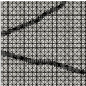
There is one regularisation parameter σ. When the data is noisy we expect that a suit-able size of σ is obtained by balancing the fidelity term with the regularisation term in the objective functional. The size of ε is determined by the need to obtain an accurate approximation of the regularised problem. We note that the thickness of the interfacial layer between bulk regions is proportional toε. In order to resolve this interfacial layer we need to choose h ε, see [23] for details. Typically reasonable results are obtained with around 8 to 10 elements across the interface. Away from the interface h can be chosen larger and hence adaptivity in space can heavily speed up computations. In fact we use the finite element toolbox Alberta 2.0, see [37], for adaptivity and we implemented the same mesh refinement strategy as in [5], i.e. a fine mesh is constructed for all variablesun_h+1, y_hn and pn_h where 0<(un_h)i <1 for at least one index i∈ {1, . . . , r} and with a coarser mesh

present in the bulk regions where (un_h)i = 0 or (uhn)i = 1 for all i ∈ {1, . . . , r}. In Figure

In our computations we found it convenient to choosehmin = ₂₅₆1 as the minimal diameter,

hmax = ₆₄1 as the maximal diameter of all elements and we set τn = 0.01/ε. The stopping

criteria we used to terminate the algorithm was the size of the residual to the first order optimality condition, i.e.k(un_h+1−un_h)/τnk ≤ 1.0e−3. For each computation we state the

number of iterations,L, required to reach this stopping criteria.

In the case r = 2 we have u2 = 1−u1 and the vector-valued Allen-Cahn inequality with

two order parameters is reduced in the computations to a scalar Allen-Cahn inequality.

Figure 1: A converged triangulation

5.1 Results with r = 2 and d= 2

In this section we see how our method compares with the one presented in [31]. In all the computations unless otherwise stated we set Ω = (−1,1)2, Jf id(Γ) := ||yΓ−yobs||2_L2_(Ω),

ε= 1

16π,a1= 3, a2 = 0.5,σ = 0.0001, Λ = 0.05 and

gh(x, y) =

  

−0.5 ifx=−1 or y=−1 0.5 ifx= 1 or y= 1.

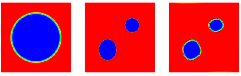
Figure 2 displays the results we obtain when using the same initial curve (a circle of radius 0.6) and objective curve (a ‘skinny’ ellitpse, x2/(0.07)2+y2/(0.5)2 = 1) that are used in Section 4.1 of [31]. In this simulation we set Λ = 0, as in [31]. The left hand plot in Figure 2 displays the initial curve, the centre plot the objective curve and the right hand plot the computed solutionun_h. The number of iterations required to reach the stopping criteria was L= 4417.

Figure 3 takes the same form as Figure 2 except that this time we compare our results with those displayed in Section 4.4 of [31]. The initial curve is again a circle of radius 0.6 while the objective curve consists of two objects

(x+ 0.35)2 (0.25)2 +

(y+ 0.35)2

(0.3)2 = 1 and

(x−0.35)2 (0.2)2 +

as in [31] we set Λ = 0. The number of iterations required to reach the stopping criteria was L = 11117. From this example we see that our phase field model successfully deals with topological change.

In Figure 4 we plot the Residual := k(un_h+1−u_hn)/τnk, J_ε,hf id(uh) := 1₂||Sh(uh)−yobsh ||2O,

J_ε,hreg(uh) :=σ

R

Ω

ε

2|Duh| 2₊ 1

2ε(1− |uh|

2₎

dxand Jε,h(uh) versus iteration number, for the

first 2000 iterations, for the computations displayed in Figures 2 and 3. From this figure we see that, in both computations, for the first 50 iterations there is a steep decrease in J,h(uh) and after that the decrease is much more gradual. We also see that the Residual

decreases at a much slower rate than J,h(uh). In Figure 5 we display two intermediate

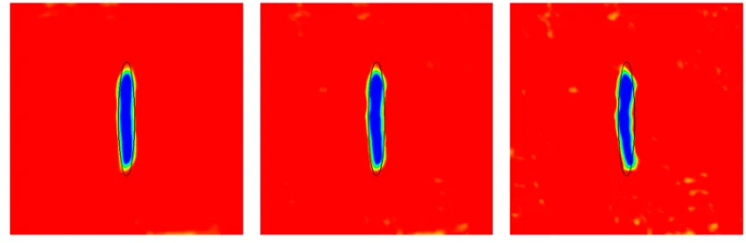
results from the set-up in Figure 2; the plots display un_h after 150 iterations (left hand plot), after 500 iterations (centre plot) and after 4417 iterations, once the iteration has converged (right hand plot). From this figure we see that after 500 iterations the solution is approximating the shape of the objective curve reasonably well although the curve is not yet defined by a well defined interfacial region.

Figure 2:Jf id(Γ) :=||yΓ−yobs||2_L2_(Ω), initial curve (left hand plot), objective curve (centre

plot),un_h (right hand plot)

Figure 3:Jf id(Γ) :=||yΓ−yobs||2_L2_(Ω), initial curve (left hand plot), objective curve (centre

plot),un_h (right hand plot)

Figure 4: Plot of J_ε,hf id(uh), Jε,hreg(uh), Jε,h(uh) and the Residual, versus the number of

iterations: results in Figure 2 (left plot), results in Figure 3 (right plot)

Figure 5: Jf id(Γ) := ||yΓ −yobs||_L22_(Ω), un_h after 150 iterations (left plot), un_h after 500

hand plot). The number of iterations required to reach the stopping criteria wereL= 4236, L= 4075 and L= 8941 respectively.

In Figure 7 we follow the authors in Section 4.5 of [31] in seeing how the value of the regularisation parameter σ effects the solution. For the initial curve we take a circle of radius 0.7 and for the objective curve we take the ellipsex2/(0.5)2+y2/(0.4)2 = 1. For the choice Λ = 0.05 we display the solutions obtained withσ = 0.01 (top centre)σ = 0.001 (top right) andσ = 0.0001 (bottom left)σ= 0.000025 (bottom centre) σ= 0.0000025 (bottom right). The number of iterations required to reach the stopping criteria were L = 3918, L= 9183, L= 5550, L= 8441 and L= 21228 respectively. From this figure we see that σ= 0.001 and σ= 0.0001 give the best approximations to the objective curve.

In Figure 8 we plot J_,hf id(uh), J,hreg(uh), J,h(uh) and the Residual for the first 4000

it-erations, for the computations displayed in Figure 7 with σ = 0.001, σ = 0.0001 and σ= 0.000025. From this figure we see that for σ= 0.001 the initial decrease in J,h(uh) is

more gradual than forσ = 0.0001 andσ= 0.000025.

Figure 6: Jf id(Γ) := ||yΓ−yobs||2_L2_(Ω), un_h obtained by taking Λ = 0.05 (left hand plot)

Λ = 0.1 (centre plot) and Λ = 0.2 (right hand plot)

In Figure 9 we show the effect that the size of|a1−a2|has on the solutionun_h. We display

the objective curve in the left hand plot and in the subsequent plots we display a zoomed in image of the approximate solution, un_h, at the end of the simulation obtained from decreasing value of|a1−a2|. We takea2 = 0.5 in all plots anda1 = 1, 3, 7 in the second,

third and fourth plots respectively. We see that the approximation to the objective curve improves when|a1−a2|increases. The number of iterations required to reach the stopping

criteria wereL= 11891,L= 5550 and L= 17072 respectively.

In Figure 10 we show the effect that the choice of O has on the solution un_h. We com-pare results obtained by takingJf id(Γ) := ||yΓ−yobs||2_L2_(Ω) to results obtained by taking

Jf id(Γ) :=||yΓ−yobs||2_L2_(∂Ω). In these simulations we set Λ = 0.02. We display the objective

curve in the left hand plot and the approximate solutionun_hat the end of the simulation ob-tained fromJf id(Γ) :=||yΓ−yobs||2_L2_(Ω)(centre plot) andJf id(Γ) :=||yΓ−yobs||2_L2_(∂Ω)(right

plot). From this figure we see that the approximation to the objective curve obtained using Jf id(Γ) :=||yΓ−yobs||2_L2_(∂Ω)is effected more by the noise than the approximation that is

Figure 7: Jf id(Γ) := ||yΓ−yobs||2_L2_(Ω), objective curve (top left), un_h obtained by taking

σ = 0.01 (top centre) σ = 0.001 (top right) and σ = 0.0001 (bottom left) σ = 0.000025 (bottom centre)σ= 0.0000025 (bottom right)

Figure 8: Plot of J_ε,hf id(uh), J_ε,hreg(uh), Jε,h(uh) and the Residual, versus the number of

Figure 9: Jf id(Γ) := ||yΓ −yobs||2_L2_(Ω), objective curve (first plot), zoomed in plot of un_h

obtained by taking (a1, a2) = (1,0.5) (second plot), (a1, a2) = (3,0.5) (third plot) and

(a1, a2) = (7,0.5) (fourth plot)

a better approximation to the objective curve than usingJf id(Γ) :=||yΓ−yobs||2_L2_(∂Ω). The

number of iterations required to reach the stopping criteria wereL= 16151 andL= 18081 respectively.

Figure 10: Objective curve (left plot),un_h obtained fromJf id(Γ) :=||yΓ−yobs||2_L2_(Ω) (centre

plot) and Jf id(Γ) :=||yΓ−yobs||2_L2_(∂Ω) (right plot)

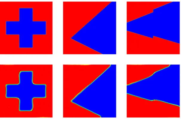
In Figure 11 we display results for three objective curves; we plot the objective curves in the upper row and the solution un_h at the end of the simulation in the lower row. In these simulations we took σ = 0.00001 and Λ = 0.005. The number of iterations required to reach the stopping criteria wereL= 12720,L= 22296 andL= 36036 respectively. From this figure we see that our method results in good approximations of the objective curves.

5.2 Results with r = 3 and d= 2

In all the computations in this section we set Ω = (−1,1)2, Jf id(Γ) := ||yΓ−yobs||2_L2_(Ω),

ε= 1

8π,a1 = 0.8,a2 = 0.2,a3 = 0.3,σ = 0.001, Λ = 0.0 and

gh(x, y) =

      

0 ifx=±1

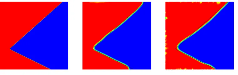
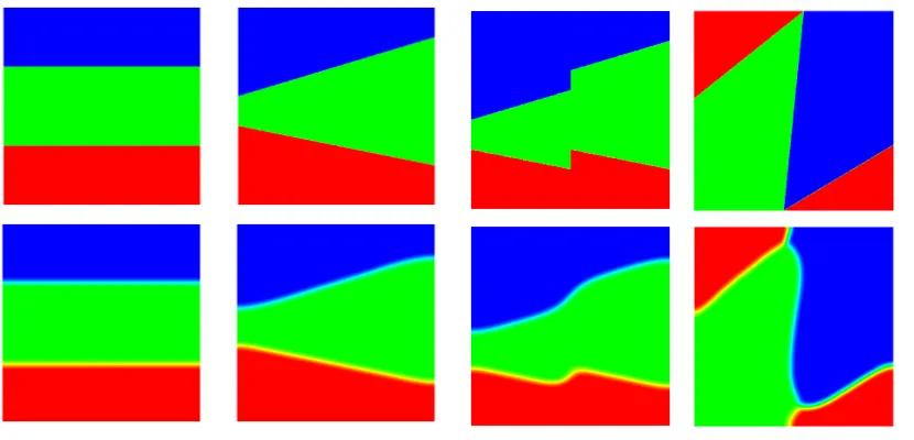
Figure 11:Jf id(Γ) :=||yΓ−yobs||2_L2_(Ω), objective curves (upper plots), un_h (lower plots)

In Figure 12 we display results for four objective curves, for each curve we took random t initial data for u0_h. We plot the objective curves in the upper row and the solution un_h at the end of the simulation in the lower row. The number of iterations required to reach the stopping criteria wereL= 10844,L= 33574,L= 31113 andL= 57373 respectively.

5.3 Summary of the computational results

The set-up of the computational examples presented in Figures 2, 3, 6 and 7 are taken from examples presented in [31]. The closeness of the approximated curve to the objective curve in the results that we present in Figures 6 and 7 is of a similar order to the results presented in [31]. In the case of Figure 2 the level set method used in [31] yields a better approximation to the skinny ellipse than our phase field model while in the case of Figure 3 our results are a substantial improvement on the ones in [31] as the level set method is unable to deal with the topological change required in this example whereas the phase field model successfully deals with it.

6

Appendix

Theorem 6.1. Let F :X→R∪ {∞} be defined by

F(u) :=

    

Z

Ω

2|Du|

2₊ 1

2(1− |u|

2₎

dx , if u∈ K;

∞ , otherwise.

ThenF

Γ

Figure 12:Jf id(Γ) :=||yΓ−yobs||2_L2_(Ω), objective curves (upper plots), un_h (lower plots)

Proof.Let us first observe that for u∈ K

F(u) = r

X

i=1

Z

Ω

2|∇ui|

2₊ 1

2(ui−u

2

i)

dx=

r

X

i=1

˜ F(ui),

where ˜F: ˜X:={v ∈L1(Ω)|0≤v(x)≤1 a.e. in Ω} →R∪ {∞} is defined by

˜ F(v) :=

    

Z

Ω

2|∇v|

2₊ 1

2(v−v

2₎

dx , ifv∈H1(Ω)∩X˜;

∞ , otherwise.

It is well–known ([33], [1]) that ˜F

Γ

→F˜ with

˜ F(v) =

    

π 8H

d−1_(∂∗_{{v= 1} ∩Ω) , ifv∈BV(Ω,{0,1});}

∞ , otherwise.

See [11, 12, 6] and the following development for the calculations leading to the factorπ/8. Let u∈ X and (uk)k∈N ⊂X an arbitrary sequence with limk→∞k = 0 and uk →u in

L1(Ω,Rr). Then (uk,i)∈N⊂X˜ and uk,i→ui inL

1_{(Ω), i= 1, . . . , r, so that}

lim inf

k→∞ Fk(uk) = lim infk→∞

r

X

i=1

˜

Fk(uk,i)≥

r

X

i=1

lim inf

k→∞

˜

Fk(uk,i)≥

r

X

i=1

˜

F(ui) =F(u)

since ˜F

Γ

→ F˜. It remains to show that for every u ∈BV(Ω,{e1, . . . , er})∩X there exists

a sequence (uk)k∈N⊂ K with limk→∞k = 0 such thatuk →u inL

1_(Ω,

Rr) and

lim sup

k→∞

We essentially follow the argument in [4]. Because of our particular choice of potential and the absence of volume constraints, the construction can be made more explicit allowing us at the same time to incorporate the condition that Pr

i=1ui(x) = 1 a.e. in Ω, which isn’t

considered in [4].

Let u ∈ BV(Ω,{e1, . . . , er})∩X, say u = Pri=1χEiei. In view of Lemma 3.1 in [4] we

can assume without loss of generality that the Ei are closed polygonal sets satisfying Hd−1_(∂E

i ∩∂Ω) = 0, i = 1, . . . , r. Lemma 3.3 in [4] implies that there exists η > 0 such

that the functionshi :Rd→R,

hi(x) :=

  

dist(x, ∂Ei), x∈Rd\Ei, −dist(x, ∂Ei), x∈Ei,

are Lipschitz–continuous onH_ηi :={x∈_Rd_{| |h}

i(x)|< η}with|∇hi(x)|= 1 a.e. in Hηi. Let

us introduce the functionϕ ∈C1(R),

ϕ(τ) :=

        

0, τ ≤0; 1

2 1 + sin τ −

π 2

, 0< τ < π; 1, τ ≥π.

Furthermore, we define χ:Rr−1 →Rr by

[χ(t)]i :=

      

1−ϕ(t1) , i= 1;

ϕ(t1)· · ·ϕ(ti−1)(1−ϕ(ti)) ,2≤i≤r−1;

ϕ(t1)· · ·ϕ(tr−1) , i=r,

wheret= (t1, . . . , tr−1). It is not difficult to verify that

χ(t) =

      

e1 , ift1 ≤0;

ei , ift1 ≥π, . . . , ti−1≥π, ti ≤0;i= 2, . . . , r−1;

er , ift1 ≥π, . . . , tr−1≥π;

(6.2)

0 ≤ [χ(t)]i ≤1, i= 1, . . . , r |Dχ(t)| ≤

c

a.e. inR

r−1_{; (6.3)}

χ(t) =

1

2 1−sin ti

− π 2

ei+

1

2 1 + sin ti

− π 2

ej, (6.4)

if 0≤ti ≤π, tj ≤0, tk ≥π, k= 1, . . . , r−1, k6=i, j and i < j.

The above function is a particular example of the function χ constructed in Lemma 3.2

in [4]. In addition we have

r

X

i=1

[χ(t)]i= 1, t∈Rr−1.

As a consequence, the function u(x) := χ(h1(x), . . . , hr−1(x)), x ∈ Ω belongs to K and

satisfies (see p. 79 in [4])

In order to analyze F(u) we introduce as in [4] fori, j= 1, . . . , r the sets Ω1:=E1,

Ω_i := {x∈Ei|hj(x)> π, j= 1, . . . , i−1}, i= 2, . . . , r;

Ω_ij := {x∈Ω|0< hi(x)< π, hj(x)<0, hk(x)> π, k6=i, j} ifi < j;

K_ij := {x∈Ω|0≤hi(x)≤π,0≤hj(x)≤π} ifi < j.

Then,

Ω\ r

[

i=1

Ω_i∪[ i<j

Ω_ij⊂[ i<j

K_ij (6.5)

and

u(x) =

    

ei, x∈Ωi;

1

2 1−sin hi(x)

− π 2

ei+

1

2 1 + sin hi(x)

− π 2

ej, x∈Ωij, i < j.

(6.6)

AbbreviatingF(u, A) :=

Z

A

2|Du|

2₊ 1

2(1− |u|

2₎

dxwe have in view of (6.5) and (6.6)

F(u)≤

X

i<j

F(u,Ωij) +

X

i<j

F(u, Kij).

It is shown in [4] that lim sup_→0F(u, Kij) = 0 for i, j = 1, . . . , r, i < j. Furthermore,

observing (6.6) and|∇hi(x)|= 1 a.e. in Ωij we obtain

|Du(x)|2=

1 22 cos

2 hi(x)

− π 2

, 1− |u(x)|2=

1 2cos

2 hi(x)

− π 2

, x∈Ω_ij, so that the coarea formula yields

F(u,Ωij) =

1 2

Z

Ω ij

cos2 hi(x) −

π 2

dx= 1 2

Z π

0

cos2 t −

π 2

Hd−1({hi=t} ∩Ej)dt

= 1 2 Z π 2 −π 2

cos2(s)Hd−1({hi =(s+

π

2)} ∩Ej)ds→ π 4H

d−1_(∂E

i∩∂Ej ∩Ω), →0.

Hence,

lim sup

→0

F(u)≤

π 4

X

i<j

Hd−1(∂Ei∩∂Ej∩Ω) =

π 8

r

X

i=1

Hd−1(∂Ei∩Ω) =F(u),

where we note that∂Ei∩∂Ejis counted twice in the second sum. In conclusion,F

Γ

→F.

Corollary 6.2. Suppose that (u)>0 ⊂ K is a sequence such that (F(u))>0 is bounded.

Then there exists a sequence k → 0 and u ∈BV(Ω,{e1, . . . , er})∩X such that uk → u

in L1(Ω,Rr).

Proof.Our assumption yields that ( ˜F(u,i))>0is bounded fori= 1, . . . , r. It is well–known

that this implies that there exists a sequence k → 0 and ui ∈ BV(Ω,{0,1}) such that

uk,i→ui inL

1_{(Ω) and a.e. in Ω, i= 1, . . . , r. Clearly,u}

k →u= (u1, . . . , ur) inL

1_(Ω,

Rr),

while it also follows thatPr

i=1ui(x) = 1 a.e. in Ω so thatu∈BV(Ω,{e1, . . . , er})∩X.

Acknowledgements

References

[1] G. Alberti,Variational models for phase transitions, an approach viaΓ–convergence, in Calculus of variations and partial differential equations (Pisa, 1996), Springer, Berlin, 2000, pp. 95–114.

[2] G. Alessandrini, V. Isakov, and J. Powell, Local uniqueness in the inverse

conductivity problem with one measurement, Trans. Amer. Math. Soc., 347 (1995),

pp. 3031–3041.

[3] H. B. Ameur, M. Burger, and B. Hackl,Level set methods for geometric inverse

problems in linear elasticity, Inverse Problems,20(2004), pp. 673–696.

[4] S. Baldo, Minimal interface criterion for phase transitions in mixtures of

Cahn-Hilliard fluids, Ann. Inst. H. Poincar´e Anal. Non Lin´eaire, 7 (1990), pp. 67–90.

[5] J. W. Barrett, R. N¨urnberg, and V. Styles, Finite element approximation

of a phase field model for void electromigration, SIAM J. Numer. Anal., 42 (2004),

pp. 738–772.

[6] G. Bellettini, M. Paolini, and C. Verdi, Γ–convergence of discrete

approxima-tions to interfaces with prescribed mean curvature, Atti Accad. Naz. Lincei Cl. Fis.

Mat. Natur. Rend. Lincei (9) Mat. Appl., 1 (1990), pp. 317–328.

[7] H. Bellout, A. Friedman, and V. Isakov, Stability for an inverse problem in

potential theory, Trans. Amer. Math. Soc.,332 (1992), pp. 271–296.

[8] H. Benninghoff and H. Garcke,Efficient image segmentation and restoration

us-ing parametric curve evolution with junctions and topology changes, SIAM J. Imaging

Sciences, 7(2014), pp. 1451–1483.

[9] L. Blank, M. H. Farshbaf-Shaker, H. Garcke, and V. Styles,Relating phase

field and sharp interface approaches to structural topology optimization,, Tech. Report

Preprint-Nr.: SPP1253-150, DFG priority program 1253 “Optimization with PDEs”, 2013.

[10] L. Blank, H. Garcke, L. Sarbu, and V. Styles, Nonlocal Allen–Cahn

sys-tems: analysis and a primal–dual active set method, IMA J. Numer. Anal.,33(2013),

pp. 1126–1155.

[11] J. F. Blowey and C. M. Elliott, The Cahn–Hilliard gradient theory for phase

separation with non–smooth free energy. I. Mathematical analysis, European J. Appl.

Math., 2(1991), pp. 233–280.

[12] ,Curvature dependent phase boundary motion and parabolic obstacle problems, in

Degenerate Diffusion, Wei-Ming Ni, L. A. Peletier, and J. L. Vasquez, eds., vol. 47 of IMA Vol. Math. Appl., Springer-Verlag, 1993, pp. 19–60.

[13] A. Boyle, A. Adler, and W. R. B. Lionheart, Shape deformation in

two-dimensional electrical impedance tomography, IEEE Trans. Med. Imaging, 31(2012),

[14] A. Braides, Γ-Convergence for Beginners, vol. 22 of Oxford Lecture Series in Math-ematics and Its Applications, Clarendon Press, 2002.

[15] C. Brett, A. S. Dedner, and C. M. Elliott, Phase field methods for binary

recovery, LNCSE, Optimization with PDE constraints, ed. R. Hoppe, 101 (2014),

pp. 25–63.

[16] M. Burger, A framework for the construction of level set methods for shape

opti-mization and reconstruction, Interfaces Free Bound.,5 (2003), pp. 301–329.

[17] T. F. Chan and X.-C. Tai,Level set and total variation regularization for elliptic

inverse problems with discontinuous coefficients, J. Comput. Phys.,193(2003), pp. 40–

66.

[18] M. Cheney, D. Isaacson, and J. C. Newell, Electrical impedance tomography, SIAM review, 41(1999), pp. 85–101.

[19] C. Clason and K. Kunisch,Multi-bang control of elliptic systems, Ann. Inst. H. Poincar´e. Anal. Non Lin´eaire, 31(2014) 1109–1130.

[20] P. Cl´ement, Approximation by finite element functions using local regularization, RAIRO Anal. Num´er., R-2 (1975), pp. 77–84.

[21] T. A. Davis,UMFPACK version 5.2. 0 user guide, University of Florida, 2007.

[22] A. DeCezaro, A. Leit˜ao, and X.-C. Tai, On multiple level-set regularization

methods for inverse problems, Inverse Problems,25 (2009), pp. 035004, 22.

[23] K. Deckelnick, G. Dziuk, and C. M. Elliott,Computation of geometric partial

differential equations and mean curvature flow, Acta Numerica, 14 (2005), pp. 139–

232.

[24] O. Dorn, E. L. Miller, and C. M. Rappaport,A shape reconstruction method

for electromagnetic tomography using adjoint fields and level sets, Inverse Problems,

16 (2000), p. 1119.

[25] O. Dorn and R. Villegas, History matching of petroleum reservoirs using a level

set technique, Inverse Problems,24 (2008), p. 035015.

[26] B. Hackl, Methods for reliable topology changes for perimeter-regularized geometric

inverse problems, SIAM J Numer Anal, 45(2007), pp. 2201–2227.

[27] J. Hegemann, A. Cantarero, C. L. Richardson, and J. M. Teran,An explicit

update scheme for inverse parameter and interface estimation of piecewise constant

coefficients in linear elliptic pdes, SIAM J. Sci. Comput.,35(2013), pp. A1098–A1119.

[28] F. Hettlich and W. Rundell,The determination of a discontinuity in a

conduc-tivity from a single boundary measurement, Inverse Problems,14 (1998), pp. 67–82.

[29] M. A. Iglesias, K. Lin, and A. M. Stuart,Well-posed Bayesian geometric inverse

[30] M. A. Iglesias and D. McLaughlin,Level-set techniques for facies identification

in reservoir modeling, Inverse Problems,27(2011), p. 035008.

[31] K. Ito, K. Kunisch, and Z. Li,Level-set function approach to an inverse interface

problem, Inverse Problems,17(2001), pp. 1225–1242.

[32] V. Kolehmainen, S. R. Arridge, W. R. B. Lionheart, M. Vauhkonen, and J. P. Kaipio, Recovery of region boundaries of piecewise constant coefficients of an

elliptic PDE from boundary data, Inverse Problems, 15(1999), pp. 1375–1391.

[33] L. Modica, The gradient theory of phase transitions and the minimal interface

cri-terion, Arch. Rational Mech. Anal.,98(1987), pp. 123–142.

[34] D. Mumford and J. Shah, Optimal approximations by piecewise smooth functions

and associated variational problems, Communications on Pure and Applied

Mathe-matics, 42(1989), pp. 577–685.

[35] L. K. Nielsen, X.-C. Tai, S. I. Aanonsen, and M. Espedal,A binary level set

model for elliptic inverse problems with discontinuous coefficients, Int. J. Numer. Anal.

Model.,4 (2007), pp. 74–99.

[36] F. Santosa, A level-set approach for inverse problems involving obstacles, ESAIM Contrˆole Optim. Calc. Var., 1 (1995/96), pp. 17–33.

[37] A. Schmidt and K. G. Siebert, Design of adaptive finite element software: The

finite element toolbox ALBERTA, vol. 42 of Lecture notes in computational science

and engineering, Springer, 2005.

[38] X.-C. Tai and H. Li,A piecewise constant level set method for elliptic inverse

prob-lems, Appl. Numer. Math., 57(2007), pp. 686–696.

[39] A. Tsai, A. Yezzi, and A.S. Willsky, Curve evolution implementation of the

Mumford–Shah functional for image segmentation, denoising, interpolation, and

mag-nification, IEEE Trans. Image Processing,10 (2001).

[40] K. van den Doel, U. M. Ascher, and A. Leit˜ao,Multiple level sets for piecewise

constant surface reconstruction in highly ill-posed problems, J. Sci. Comput.,43(2010),