Abstract— Most sensor network deployments are 2-tiered and are preceded by a topology study to determine the optimal location of sensors and relays. Sensors form the leaves in a 2-tiered network and do not participate in the routing. A plot of the best path from each of the leaves to the sink reveals the network topology to be hierarchical in nature. The AODV routing algorithm was designed for highly mobile nodes and is not directly suitable in a hierarchical sensor network where the sensors and relays are predominantly static. The Hierarchical routing as implemented by ZigBee’s Cskip does not support fault tolerance
and has a restriction on the network depth. In this paper, we present a probability based routing algorithm that merges the structure of a hierarchical tree with the flexibility of AODV. As devices join a network, they are given an address to satisfy the hierarchical property. Here, the address generation is made based on the expected number of devices to join the network. When a condition occurs where the hierarchical property can no longer be supported, a route table entry, similar to AODV, is created only for this non-conforming node. The mechanism of making route table entries has inherent support for fault tolerance. The completeness of the algorithm is determined theoretically and by an exhaustive simulation in C++. We provide the results of the memory requirement, the sensitivity to the network deployment probability distributions and the probability of address duplication.
Index Terms—Hierarchical Routing, ZigBee.
I. INTRODUCTION
The wireless sensor networks comprise of sensors and actuators that are designed to run on batteries for prolonged periods of time. These devices and such networks need to support low data rates and the computational capability is restricted [1]. The devices compute routes among themselves for multi hop data dissemination to a particular device generally designated as a sink. Further, the devices are typically deployed in harsh and unconditioned environments where unpredictable events like battery depletion or environmental disturbances can lead to failures, thereby restricting effective operations. Thus, important aspects of a wireless sensor network are its capability to achieve an efficient routing scheme and the degree of robustness.
The topology of a wireless sensor network is the logical route taken by a packet moving from the source to the destination. The topology construction, through the routing scheme, is the function of the NTW (network) layer in the 7 layer OSI stack. In multi-hop wireless systems, the topology can be of two forms – a mesh or a hierarchical tree. In a mesh topology, wireless devices maintain routes to every device in
Manuscript received August 1, 2008. This work was supported in part by the Infosys Fellowship Grant.
Anurag D is with the Indian Institute of Management Calcutta, Kolkata, India 700104 (e-mail:[email protected]).
Somprakash Bandyopadhyay is with the Indian Institute of Management Calcutta, Kolkata, India 700104 (e-mail:[email protected]).
its communication range while in a hierarchical network the device maintains a route to only its parent and its children. The algorithms for routing and fault tolerance are designed to develop an efficient path for the multi-hop routes during normal operation and in the event of a node/link failure. The widely studied and implemented routing protocol for wireless mesh networks is AODV (Ad-hoc On-demand Distance Vector) [2]. AODV was developed for mesh networks that have highly mobile nodes where routes are broken easily. The hierarchical tree topology has received little attention with the most notable implementation support coming from the ZigBee [14] stack. Here an addressing scheme called Cskip, is
utilized to provide addresses to the nodes. The hierarchical topology requires no routing tables to be generated as the node addresses are sufficient to make the routing decisions. The hierarchical topology has been shown to provide the most efficient routing [9]. However, it has no support for fault tolerance. Further, the Cskip algorithm faces a severe address
wastage problem [1], where extended multi hop reach is restricted. These aspects are elaborated in section 2.
II. MOTIVATION
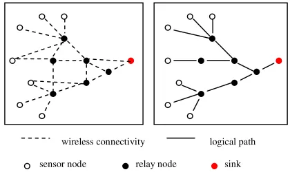
[image:1.612.321.531.575.700.2]We study the deployment of a wireless sensor network with sensors being placed at particular points in the region to be monitored. The sensed parameters include temperature, vibration and (harmful) gases. The sensors are placed at pre-determined points and it is well understood by the sensor network user that the sensed parameters correspond to the point of the sensor location rather than the region (for e.g. a vibration sensor is placed on a specific asset and is immobile). The sensed information is to be transported to the centralized data repository located at the sink. The sensors do not participate in the packet forwarding and relays are placed at appropriate locations to transmit the data in a multi-hop fashion to the sink. Such networks are known as 2-tiered and are the most common form of sensor network deployment.
Figure 1. A mesh network reduces to a hierarchical minimum spanning tree when data communication is required only between the nodes (sensors and
relays) and the sink.
Achieving Fault Tolerance and Network Depth
in Hierarchical Wireless Sensor Networks
Anurag D and Somprakash Bandyopadhyay
The data propagates from the sensors to the sink and vice-versa. There is no requirement for one sensor to communicate to another sensor, or one relay to communicate to another relay. If we plot the topology of the best path (the metric can be hop counts, signal strength, etc) from the sensors to the sink, it would result in a hierarchical structure as shown in figure 1. This is analogous to the minimum spanning tree.
The AODV routing algorithm builds the route tables by a flooding the network with RREQ control packets. These control packets are costly since all devices are battery powered and packet transmissions are the biggest source of energy dissipation. In case of node failures, RRER control packets are generated and subsequent RREQ packets to establish the new route.
The Cskip algorithm used by ZigBee allocates addresses to
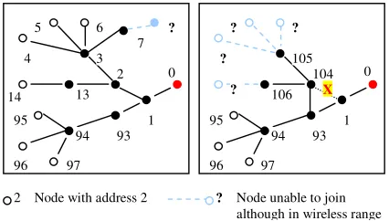
each node such that routing can be made without having to generate any routing table. It earmarks each node to have a fixed number of children. This fixed allocation restricts the total depth (number of hops) that the network can support. For example, if every relay is expected to support upto 9 relays as its children, the maximum depth is 4. As shown in figure 2(a), a device at depth 5 cannot join the network. The ZigBee hierarchical routing algorithm also does not support fault tolerance. When a node in the network goes down, all its child nodes look for a new parent. If a new parent is found, the child node’s address changes. This in turn results in the changing of the address of all the children of the child node and continues recursively till the leaves of the network. While obtaining a new parent, if the depth of the node increases, devices that were part of the network earlier may not be able to join. This is shown in figure 2(b). The link between devices numbered 2 and 1 goes down. Device 2 connects to device 93 and is reassigned an address of 104. Note that its depth has also increased. As a consequence the children of 2, are renumbered as 105 and 106 while the sensors, earlier numbered 4, 5, 6 and 14 are no longer able to be part of the network although they are in wireless range. This is due to the address wastage of Cskip where it has earmarked addresses for
non-existent devices.
Figure 2(a). The nodes given addresses according to Cskip with each relay expected to support upto 9 children. In such a case, depth larger than 4 is not possible. (b). Break in link between 2 and 1 (shown as X) results in 3 devices being assigned a new address and 4 sensors no longer part of the network.
As a further example, if the number of child relays a relay is able to support is set to 5, the maximum depth is 6. Similarly, if the max child relay is set to 15, the maximum depth is 4. In this paper, we develop a routing algorithm that includes both the properties of the hierarchical as well as AODV protocols. As devices join a network, they are given address to satisfy the hierarchical property. Here, the address
generation is made based on the expected number of devices to join the network. As the network grows with more devices joining, the expected number of devices to join falls. Thus the address space (and wastage) is reduced as the network grows. When a condition occurs where the hierarchical property can no longer be supported, a route table entry, similar to AODV, is created only for this non-conforming node. This route table entry is also created when a node/link fails thus preventing other nodes from having to change their addresses or depth. Our routing algorithm can be tuned to the probability distribution of node deployments. For example, a dense network with low depth can be tuned to a uniform distribution. In case of a network with long chains (effectively large depth) a geometric distribution can be used. We term our probability based routing algorithm as a hybrid of the hierarchical and AODV algorithms.
The aim is to achieve a routing algorithm suitable for 2-tiered wireless sensor network which has a low control packet overhead and at the same time supports large network depth and is fault tolerant
III. RELATED WORK
Numerous studies have been made on achieving efficient routing in wireless mesh networks. Significant work includes flooding [11], the AODV protocol [2] and the Location Aided Routing (LAR) protocol [7]. In hierarchical routing, the addresses of the nodes play a critical role as they decide the routing decision. A hierarchical address allocation is made by the Cskip algorithm of ZigBee [14]. Here, a device joins the
network by requesting an address from a particular device, now designated as the parent. The parent gives an address according to the equation:
) (d C A
Anew = parent + skip (1) where d is the depth of the child and Cskip is the maximum
number of devices that can join under all the other children of the parent. This scheme looks to reserve addresses in the event a node joins at a particular level. Since this cannot be predicted apriori, most reserved addresses are never utilized restricting devices to join in an already dense area. This restricts the depth of the network. The Cskip algorithm was
mainly expected to be used in a star network where typically there is no multi hop data transmission. However, this address wastage problem has been thought about in the latest ZigBee specification made available to the general public on January 2008 [14]. The specification in addition to Cskip, has included
support for a stochastic addressing scheme where addresses are assigned in a random fashion. Here, there is no guarantee for uniqueness of the address and address conflict negotiation mechanisms are defined. Stochastic addressing automatically implies AODV mechanism is used for routing.
Work on optimized deployment and fault tolerance has recently gained momentum. Sensor coverage problems [10, 12] have looked at placing enough sensors to cover the entire area of deployment. Once an initial topology is obtained, additional routers (or relays) can be placed to achieve fault tolerance [6, 13]. A (k-1) fault tolerant network is one where every node is k connected and the network remains connected even after k-1 node failures. Existing sensors are modeled as a unit disk graph with the sensors designated as a vertex. The goal is have every vertex k-connected. Thus these
Node with address 2 0
1 2
93 3
13
94 95
6 5
4
14
96 97
7 ?
0
1 104
93 105
106
94 95
? ?
?
?
96 97
2 Node unable to join
although in wireless range ?
[image:2.612.78.291.499.620.2]optimization schemes augers well with the hierarchical topology, however no work has been made at developing an addressing and routing scheme for wireless hierarchical networks that support fault tolerance.
IV. PROBLEM FORMULATION
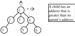
[image:3.612.126.248.273.332.2]The sensor network comprises of one sink, multiple sensors that are fixed (immobile) and form the leaves of the network. Routers are placed to relay the data from the sensors to the sink and vice-versa. Each of the sensors, routers and the sink are homogeneous and have a fixed radius of transmission. The network grows from the sink towards the leaves. The sink is the first device in the network to come up and takes the address of 0. Subsequent routers/sensors request an address from an already associated device in its range. Our algorithm provides this address in an intelligent way. There is no apriori information of which device would come up next and hence the algorithm is generic and supports any structure of the topology. A sample topology is shown in figure 3.
Figure 3. A sample hierarchical topology.
The address of a device uniquely identifies it in the network. Further, the address is used to make routing decisions. For example, in figure 3, if node numbered 1, receives a packet with destination address 3, it must be able to decide to which of its children (among 2, 7 and 4) the packet must be forwarded, to ensure the packet reaches the destination. In most routing protocols, typified by AODV, the node needs to maintain a list guiding it on the network topology. However, in the case of a hierarchical network, the node addresses are assigned in a way to ensure routing decisions can be made. We define this decision of a node as its routing strategy S. Note that the strategy, S, must be simple enough to run on resource (computational) constrained devices in acceptable time. Further, the strategy must be the same for all the nodes, i.e., referring to figure 3, node 1 cannot make a routing decision unless it knows the strategy followed by its children. We now define the strategy, for our proposed algorithm, S as in (2) and a new requesting device is given an address according to (3).
ess ParentAddr dresses
ChildrenAd
S: > (2)
) (
max E n
A
Anew = + (3)
Where Amax is the maximum address reachable through the
parent, E ( ) is the expected value of the probability distribution and n is the number of devices left to join the network. The algorithm thus calculates the expected number of devices for a particular distribution function, rather than earmark the worst case solution as in Cskip. Further, in cases
where the number of devices joining exceeds the expected value, an exception list is maintained which is the route entry only for the non conforming device similar to the AODV entry. Thus, our addressing algorithm, maintains as much as possible, the hierarchical structure. However, in cases where it is not possible, an exception is created and saved as a list.
The algorithm essentially is a merge of the structured hierarchical network and the completely unstructured AODV mechanism.
Table 1. Notations used.
Notation Meaning
N Expected number of devices in a network. (user generated)
n current number of devices in the network that have to yet join (out of N)
E(n) Expectation for a given probability distribution generating the number of devices expected to join the given device
p(x) probability of x devices joining
The Hybrid Routing Algorithm
0: Node Start-up (switched on). Perform Initialisation. 1: Perform Channel Scan.
If no devices found in range, goto 1 else set my_parent = device
with strongest signal strength
2: Send Associate_request to my_parent
3: If associate_response received from my_parent
set my_address = address from associate response
4: If Associate_request received, then
If I am not PAN coordinator then
send new_address_request to my_parent
with P=my_address as parameter
else
Calculate E =num of devices expected to join.
set N = last child address+ E
Send Associate_response with N as the new address
5: If new_address_request received from any node R
If I am not PAN coordinator then
forward new_address_request to my_parent
else
calculate E = number of devices expected to join under P
set N = last child address of P + E
If N breaks hierarchical routing, create route table entry
with N as destination and R as next_hop
reply with new_address_response; P, N as parameters
6: If new_address_response received from any node R
If N breaks hierarchical routing, create route table entry with
destination as N and R as next_hop
If my_address = P then
send associate_response with N as address
7: If data packet for routing is received
If destination exists in route table forward to next_hop else
forward according to hierarchy
8: If packet sending to my_parent fails
perform channel scan
set my_parent=device with strongest signal if device is not reachable through me
send route_update to my_parent with my_address as parameter
9: If route_update received from any node R
If address breaks hierarchical routing, create/update route table entry with address as destination and next hop as R
forward route_update to my_parent 1
2
3
4
5 6
7
Lemma 1: Defining the routing strategy as in (2) and the addresses as in (3), newly assigned addresses cannot invalidate the already setup routing scheme.
Proof: A sample topology is shown in figure 4. Assume an existing node with an address “A”. We define all the addresses of the nodes (parents) connecting “A” from the sink as “Pk”, where k =1 to D, D= depth of A. Let a new node
joining the network get an address “N”. Let “Qk” be the list of
addresses of the nodes connecting “N” to the sink with k=1 to D, D = depth of N. Select the node common to Pk and Qk that
has the highest address. (There will be atleast one node common to Pk and Qk). Let this node be denoted C. Let the
node under C with the largest address be denoted as Cn. The
routing to A will fail if N joins the network at C and N < A. However, N > Cn and Cn >= A by (3). Thus the routing to A is
[image:4.612.130.251.231.327.2]preserved.
Figure 4.Sample topology for Lemma I
Lemma II: The upper bound on the number of exceptions on a node (hence the maximum requirement of memory for route tables) with “N” devices in the entire network is given by:
− < − − + =
− −
∑
∑
= −
=
otherwise
N E i N E if
p
where p
N
k
i k
N
k k
0
) 3 ( ) 4 ( 2 1
) 3 (
1 5
1
Proof: The worst case scenario for the exceptions is as shown in figure 3. The maximum exceptions needed when E (x) = 1 for all values of x, will be N – 3, where N is the number of devices expected in the entire network. No exceptions will be needed for devices whose addresses are less than E(N-3).
Figure 5.Sample topology for Lemma II and III.
Lemma III: The worst case address wastage in a network, expected to hold “N” devices, is given by:
) 3 ( ) ( 1
3
− − −
∑
−=
N i N E
N
i
Corollary: The worst case number of devices that can be supported by a network with a 16 bit address is given by:
where K
∑
= ==
−
K ii
i
K
E
3
16
2
)
(
Proof: From figure 3, the worst case in terms of address wastage occurs when all devices look to join the PAN coordinator. The third device would join with an address space of E(N-3) - 1. The fourth device would join with an
address space of E(N-4) - 1. This address space would be wasted if no device joins the network at the second, third, etc device and instead join at the first device. Thus the maximum address wastage is the sum of the address space. Similarly, the last device with an address equal to the sum of all the address space must be just less than
2
16to be successfully associated. Calculating the value of N for such a scenario gives the worst case number of devices. For example, if the distribution of the network formation is considered to be uniform, the worst case number of devices turns out to be 31706 and the probability of such a worst case network occurring turns out to be128946
10 )! 31706 (
1 −
≈
. Support for Large Network Depth:
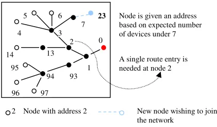
In this section, we show pictorially how the algorithm handles networks of large depth. Considering the example shown in figure 2(a), the new node must be given an address to join the network. However, no address will satisfy the hierarchical property. We therefore give it an address based on the expected number of devices under node 7. The new address creates route table entry only at node 2. Thus a single route table entry is sufficient for routing. As shown in figure 6, assume the new node is given an address of 23.
[image:4.612.319.530.419.543.2]A packet destined for node 23 is routed as follows. At node 1, the hierarchical strategy eqn. (2) implies the packet must be forwarded to node 2. Similarly, the hierarchical property at node 2 implies the packet must be forwarded to node 13. However, the route entry is present at node 2 directing the packet to node 3. The hierarchical property is satisfied at node 7 as well thus reaching the packet to node 23.
Figure 6. Support for large network depth
Support for Fault Tolerance:
The hybrid addressing topology has inherent capability to support fault tolerance. In the event of a node failure, a node selects the new parent that would enable it to reach the sink. It presents its address to the new parent. The new parent in turn, checks for the hierarchical property and creates/updates route table entries if needed and forwards the packet to its parent. This can be considered similar to the AODV style RREQ (route request) and RREP (route reply) messages.
An example is shown in figure 7. The link between nodes 2 and 1 break and node 2 joins node 93. Since all of the addresses under node 2 are less than 93, a route table entry is required for each of the 7 devices at node 1. However, no route table entries are needed at any other node since the hierarchical property is satisfied elsewhere.
Node with address 2 0
1 2
93 3
13
94 95
6 5
4
14
96 97
7 23
2 New node wishing to join
the network Node is given an address based on expected number of devices under 7
A single route entry is needed at node 2
E(N-6) E(N-3)
0
1
2
Maximum Exceptions occur when maximum possible devices join under a single parent.
E(N-5) Cn
A N
C
Figure 7.Support for fault tolerance
V. IMPLEMENTATION AND EVALUATION
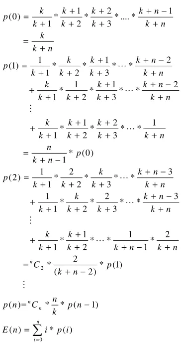
[image:5.612.323.529.281.385.2]We implemented the routing scheme assuming a uniform distribution for node generation. A node can join any of the previously joined nodes with equal probability. Referring to figure 11, “k” denotes the number of nodes in the leg where the new device is joining and “n” denotes the number of devices yet to join. The expected number of devices under a particular node is calculated in O(n) time. The appendix provides the implementation details.
We compare the above address allocation algorithm with the memory requirement in AODV for storing the route tables. Intuitively, our scheme must show a significant improvement since the address allocation happens in an intelligent way where the hierarchical structure is maintained as much as possible. In cases where this is not possible, the AODV style route table for only the exception device is stored. An additional overhead in our scheme is a single unit to store the maximum address under the device as is needed by (3).
Memory Requirement
0 0.5 1 1.5 2 2.5 3 3.5 4 4.5
25 50 75 100 125 150 175 199
Number of nodes
M
e
m
o
ry
(
A
v
g
)
0 50 100 150 200 250
M
e
m
o
ry
(
M
a
x
)
[image:5.612.79.289.456.568.2]AODV (Avg) Hybrid (Avg) AODV (Max) Hybrid (Max)
Figure 8. Memory Requirement for network topology generated through a uniform distribution.
The simulation was carried out in C++ where the node placement is randomized. The placement of a new node was studied in two settings. In one, a uniform probability distribution of node placement was done. Here, a new node N would have equal probability to choose any of the previously deployed nodes as its parent. In the second setting, a geometric probability distribution was used. Here a new node N has maximum probability of choosing the last deployed node as its parent and the probability of choosing an earlier deployed node falls proportionately. The geometric distribution is a more realistic representation of the practical scenario. Once a random network topology is generated, the memory needed for AODV and the hybrid scheme is
calculated for the same topology. We calculate the network average (denoted as AVG) and the node average for the node with the biggest route table (MAX).
The Hybrid routing, as expected, clearly outdoes the AODV scheme on both the network average and the node average counts. The hybrid scheme requires around 50 % less memory. Figure 9 gives the performance of the AODV protocol and the Hybrid protocol for the geometric distribution of topology generation. Interestingly, AODV suffers significantly compared to the Hybrid algorithm. This can be explained by noting that the topology would be of larger depth on most occasions. In a uniform distribution, the topology would be lower in depth and wider in width. Therefore in uniform distribution there would be more nodes that have no children. When a node has no children, it needs no route table. However, for a geometric distribution, nodes with no children are smaller in number thus leading to a larger average requirement of memory. The hybrid algorithm is more comfortable with the geometric distribution as increase in depth leads to a lower increase in the number of exceptions.
0 5 10 15 20 25
25 50 75 100 125 150 175 199
number of nodes
m
e
m
o
ry
(
a
v
g
)
AODV ( avg ) uniform AODV ( avg ) geometric Hybrid ( avg ) uniform Hybrid ( avg ) geometric
Figure 9. Memory requirement for AODV and Hybrid under uniform distribution and geometric distribution (p=0.8)
Address Clashes
The hybrid algorithm assigns addresses in a deterministic manner; i.e. for the same topology generated in the same order will lead to the same addresses being calculated. Thus we could simulate our scheme to check for the duplication of addresses. As seen in figure 10, the scheme performs rather poorly on this front. The geometric distribution has an approximate clash rate of one in three.
0 20 40 60 80 100
25 50 75 100 125 150 175 199
Number of Nodes
N
u
m
b
e
r
o
f
c
la
s
h
e
s
(
a
v
g
[image:5.612.323.530.530.636.2]) Hybrid, geom dist Hybrid, unif dist
Figure 10.Number of address duplication for hybrid scheme.
The poor address uniqueness property of our hybrid scheme immediately motivates us in incorporating small stochastic elements.
ε
+ += ( )
max E n
A
Anew (4)
Node with address 2
0
1 2
93 3
13
94 95
6 5
4
14
96 97
2 Node which is unable to
join in ZigBee X Nodes continue to
retain their earlier address.
where
ε
is a stochastic error which is a function of the number of devices in the network. Note, for Lemma I to hold,ε
must necessarily≥
0. We plan to explore such a scheme in [image:6.612.69.300.101.215.2]our future work.
Table 2. Simulation Setup.
Simulation Environment C++
Number or nodes in network 25 to 200, in steps of 25 Location of nodes
(Sensitivity Runs)
pseudo random uniform distribution
pseudo random geometric distribution with p=0.8 Number of runs 100 for each network size
VI. CONCLUSION
Our proposed hybrid algorithm for addressing and routing in hierarchical networks borrows concepts from Cskip of
ZigBee and AODV protocol. By merging the flexibility of AODV and the structure of Cskip, we achieve significant
improvements in terms of memory needed for route tables over AODV and flexibility and support for fault tolerance over Cskip. Unlike AODV based addressing, where node
addresses are given in a stochastic manner, we give addresses in a clever scheme where the hierarchical structure is maintained as much as possible. Where addresses can be maintained in a hierarchy, there is no need for routing tables. In cases, where the hierarchy breaks, we maintain a route entry only for the non-conforming node. This exception is the overhead in our scheme. Simulation results have shown significant reduction in the routing tables (around 50%) and much better scalability with network size than AODV. The simulation also shows the rather poor address uniqueness property of our scheme (around 33%). We have identified a mechanism to abate this concern through the use of small stochastic elements.
We look to explore the inclusion of the stochastic components in our algorithm and study the improvement in the uniqueness property in our future work. Work has also been made in a practical implementation. We seek to make a large scale implementation and study the ease of deployment. The impressive gains of our scheme inspire us to develop the algorithm into practical implementations.
VII. REFERENCES
[1] Akyildiz, I.F., Xudong Wang: A Survey on Wireless Mesh Networks, IEEE Communications Magazine, September 2005.
[2] A. Wheeler, “Commercial Applications of Wireless Sensor Networks using ZigBee”, IEEE Communications Magazine, April 2007. [3] C. Perkins, E. Royer, “Ad hoc On-Demand Distance Vector Routing”,
IEEE Workshop on Mobile Computing Systems and Applications, 1999
[4] C.S. Raghavendra, A. Avizienis and M.D. Ercegovac, “Fault Tolerance in Binary Tree Architectures,” IEEE Transactions on Computers, 1984.
[5] G. Lewis et al, “A System for Simulation, Emulation, and Deployment of Heterogeneous Sensor Networks,” SenSys ’04.
[6] ITU Report on Internet of Things – Executive Summary: www.itu.int/internetof things/
[7] J. L. Bredin, E. D. Demaine, M. Hajiaghayi, D. Rus “Deploying Sensor Networks with Guaranteed Capacity and Fault Tolerance,” MobiHoc 2005.
[8] K. Young-bae and N. Vaidya, “Location-aided Routing (LAR) in Mobile Ad Hoc Networks”, ACM MobiCom, 1998.
[9] M. B. Lowrie and W. K. Fuchs, “Reconfigurable Tree Architectures Using Subtree Oriented Fault Tolerance,” IEEE Transactions on Computers, October 1987
[10] R. Peng, S. Mao-heng, Z. You-min, “ZigBee Routing Selection Strategy Based on Data Services and Energy-balanced ZigBee Routing”, IEEE Asia-Pacific conference on Services Computing ,December 2006.
[11] S. Toumpis, L. Tassiulas, “Optimal Deployment of Large Wireless Sensor Networks”, IEEE Transactions on Information Theory, 2006. [12] W. R. Heinzelman, J. Kulik, H. Balakrishnan, “Adaptive Protocols for
Information Dissemination in Wireless Sensor Networks”, ACM MobiCom, 1999.
[13] W. You-Chiun, H. Chun-Chi, T. Yu-Chee, “Efficient Placement and Dispatch of Sensors in a Wireless Sensor Network”, IEEE Transactions on Mobile Computing, 2008.
[14] X. Han, X. Cao, E. L. Lloyd, S. Chien-Chung, “Fault Tolerant Relay Node Placement in Heterogenous Wireless Sensor Networks,” InfoCom ’07.
[15] ZigBee Alliance: www.zigbee.org
APPENDIX
Calculation of E(n) given the expected number of devices in the network (N) and number of devices yet to join (n).
Figure 11. Calculation of E(n) when a new device joins.
∑
= = − = − + = + − + + + + + + − + + + + + + − + + + + = − + = + + + + + + + + − + + + + + + + − + + + + + = + = + − + + + + + + = n i n n n i p i n E n p k n C n p p n k C n k n k k k k k n k n k k k k k n k n k k k k k p p n k n n k k k k k k k n k n k k k k k k n k n k k k k k k p n k k n k n k k k k k k k p 0 2 ) ( * ) ( ) 1 ( * * ) ( ) 1 ( * ) 2 ( 2 * 2 * 1 1 * * 2 1 * 1 3 * * 3 2 * 2 * 1 1 3 * * 3 * 2 2 * 1 1 ) 2 ( ) 0 ( * 1 1 * * 3 2 * 2 1 * 1 2 * * 3 1 * 2 1 * 1 2 * * 3 1 * 2 * 1 1 ) 1 ( 1 * .... * 3 2 * 2 1 * 1 ) 0 ( M L M L L L M L LA new device (shown in grey) joins the network. K devices
[image:6.612.312.494.399.744.2]