Quiet Zone Design in Broadband Diffuse Fields
Wen-Kung Tseng
Abstract— In this paper design of quiet zones in broadband
diffuse fields has been present by using the method of acoustic pressure minimization over various spaces and frequencies. The technique is squared acoustic pressure minimization. The theory and simulations of pressure minimization over space and frequency using two-channel and three-channel systems are presented. The work presented in this paper is the second part of the study and we focus on diffuse primary fields with two and three secondary sources. The first part of the study concerned with a plane wave primary field only. A constrained minimization of pressure is also introduced in this paper, to control pressure at various spaces and frequencies. The results show that a good attenuation is achieved at the microphone location or desired range over space and frequency using a two-channel system. However, a better performance could be achieved using a three-channel system.
Index Terms—active control system, broad-band diffuse
fields, acoustic pressure, diffuse primary fields, constrained minimization.
I. INTRODUCTION
Previous work on active control of diffuse fields investigated the performance of pressure attenuation for single-tone diffuse field only which was produced by single frequency [1, 2, 3, 4, 5]. Recent work on broad-band diffuse fields only concentrated on analysis of auto-correlation and cross-correlation of sound pressure [6, 7, 8]. However there is no paper related to active control of broad-band diffuse fields. Therefore this paper will analyze the sound field and investigate the performance of active control of broadband diffuse fields.
Recent studies have shown that minimizing the acoustic pressure or vibration over a desired region in space using a two-norm strategy for a single-tone disturbance or some bending modes of vibration could produce larger zones of quiet [6, 7] or obtain vibration reduction throughout the entire structure [8], and could achieve an improved spatial performance. Therefore the minimization of acoustic pressure over space and frequency is desirable for achieving a good performance[9], e.g. high attenuation of the broad-band disturbance over a large space. Previous works on active control of broadband disturbance over space and frequency only concerned with a plane wave primary field [9, 10]. However, the work presented in this paper concerned with broad-band diffuse primary fields. Recent work on broad-band diffuse fields only concentrated on analysis of
auto-correlation and cross-correlation of sound pressure [11, 12, 13]. However there is no paper related to active control of broad-band diffuse fields. Therefore this paper will analyze the sound field and investigate the performance of active control of broadband diffuse fields. Moreover a constrained minimization of acoustic pressure is introduced, to achieve a better control of acoustic pressure in both frequency and space. The paper is organized as follows. First, the mathematical model of broad-band diffuse fields is derived. Second, the theory of active control for broad-band diffuse fields is introduced. Then, simulation results of actively controlling broad-band diffuse fields are presented. Finally the conclusions are made.
Manuscript received December 20, 2008. This work was supported by the National Science Council of Taiwan, the Republic of China, under project number NSC-96-2622-E-018-004-CC3.
W-K Tseng is with the Graduate Institute of Vehicle Engineering National Changhua University of Education, Changhua City, Taiwan (phone: +886-47232105; e-mail: [email protected]).
II. THEWAVEMODELOFBROADBANDDIFFUSE SOUNDFIELDS
Previous work used the wave model for a pure tone diffuse field, which is comprised of large number of propagating waves arriving from various directions [14, 15].
In our study we chose 72 such incident plane waves together with random amplitudes and phases to generate an approximation of a diffuse sound field in order to coincide with that in previous work. Thus the diffuse sound field was generated by adding together the contributions of 12 plane waves in the azimuthal directions (corresponding to azimuthal angles ϕL = L× 300, L=1,2,3, . . . , 12) for each of
six vertical incident directions (corresponding to vertical angles θK = K× 300 for K = 1, 2, 3, . . . , 6). The net pressure in
the point (x0,y0) on the x-y plane due to the superposition of
these 72 plane waves was then calculated from the expression
Pp(x0,y0, k) = (a
L L K K
=
=
∑
∑
1 1
max max
KL +jbKL) sinθK exp(jk(x0sinθK
cosϕL + y0sinθKsinϕL)) (1)
in which both the real and imaginary parts of the complex pressure are randomly distributed. The values of aKL and bKL
are chosen from a random population with Gaussian distribution N(0,1) and the multiplicative factor sinθK is
included to ensure that, on average, the energy associated with the incident waves was uniform from all directions. Each set of 12 azimuthal plane waves arriving from a different vertical direction θK , is distributed over a length of
2πr sinθK , which is the circumference of the sphere defined
by (r,ϕ,θ) for θK. This results in higher density of waves for
smaller θK , and thus more energy associated with small θK .
To ensure uniform energy distribution, the amplitude of the waves is multiplied by sinθK , thus making the waves coming
from the ‘‘dense’’ direction, lower in amplitude. Substituting
k= f
c
π
Pp(x0, y0, f) = ∑ ∑ (a = = max K 1 K max L 1 L
KL +jbKL) sinθK exp(j f c
π
2 (x0sinθK
cosϕL + y0sinθKsinϕL)), (2)
Where f is frequency and c the speed of sound. Equation (2) is the wave model of the pure tone diffuse field since only the single frequency plane wave arriving from uniformly distributed directions is considered. If the diffuse field is broad-band within the frequency range of fl and fh, then the wave model of the broad-band diffuse field Ppb can be expressed as ∑∑ ∑ = = = + + = − fh fl f K K L L L K L K K KL KL
pb fx y
c j jb a fh fl y x P max 1 max 1 0 0 0
0 ( sin cos sin sin ))
2 exp( sin ) ( ) , ,
( θ π θ ϕ θ ϕ (3)
where fl-fh is the frequency range from fl to fh Hz. Equation (3) will be used for broad-band diffuse primary sound field in this work. Next we will describe the formulation of the control method, and their use in the design of broad-band diffuse field quiet zones.
III. THEORYOFPRESSUREMINIMIZATIONFOR BROAD-BANDDISTURBANCE
In this section we present the theory of actively controlling a broad-band diffuse field. The basic idea is to minimize acoustic pressure over both space and frequency. Figure 1 illustrates the configuration of acoustic pressure minimization over space and frequency. In this work, the case of a one-dimensional space and a broad-band diffuse primary field derived in equation (3) is considered and the secondary sources are located at the origin and (-0.1m, 0) point. A microphone can be placed at the desired zone of quiet or other locations close to secondary monopoles. The secondary sources are driven by feedback controllers connected to the microphone. The microphone detects the signal of the primary field, which is then filtered through the controllers to drive the secondary sources. The signals from the secondary sources are then used to attenuate the primary disturbance at the pressure minimization region.
The x-axis in Fig. 1 is a one-dimensional spatial axis, which could be extended in principle, to 2 or 3D. The desired zone of quiet can be defined on this axis where a good attenuation is required. The y-axis is the frequency axis where the control bandwidth could be defined. The acoustic disturbance is assumed to be significant at the control frequency bandwidth. The shadowed region is the pressure minimization region, i.e., the desired zone of quiet over space and frequency. The region to the right of the pressure minimization region is the far field of the secondary sources, with a small control effort, and thus a small effect of the active system on the overall pressure. The region to the left of the pressure minimization region is the near field of the secondary sources, which might result in the amplification of pressure at this region. To avoid a significant pressure amplification a pressure amplification constraint should be included in the design process using a constrained optimization. The regions above and below the pressure minimization region represent frequencies outside the bandwidth. Due to the waterbed effect [16], a decrease in the disturbance at the control bandwidth will result in
amplification outside the bandwidth. Therefore, pressure amplification outside the bandwidth must be constrained in the design process.
The feedback system used in this work is shown in Fig. 2 and is configured using the internal model control [17] as shown in Fig. 3, where P1 is plant 1, the response between the
input to the first monopole and the output of the microphone,
P1o is the internal model of plant 1, P2 is plant 2, the response
between the input to the second monopole and the output of the microphone, P2o is the internal model of plant 2, Ps1and Ps2 are the secondary fields at the field point away from the
first and second monopoles respectively, d is the disturbance, the broad-band diffuse field, at the microphone location, ds is
the disturbance at the field point away from the microphone, and e is the error signal. In this work, P1o is assumed to be
equal to P1 and P2o is equal to P2. Therefore the feedback
system turns to a feedforward system with x=d, where x is the input to the control filters W1 and W2. .
It is also assumed that the secondary and primary fields in both space and frequency, are known, and although a microphone is used for the feedback signal, pressure elsewhere is assumed to be known and this knowledge is used in the minimization formulation. Although it is not always practical to have a good estimate of pressure far from the microphone, this still can be achieved in some cases using virtual microphone techniques[14] which provide a sufficiently accurate estimate of acoustic pressure far from the microphone.
The secondary fields at the field point away from the secondary monopoles could be written as[3]:
P r f A r e
s
j fr c
1 1
1
1
2 1
( , )= − π / , (4)
P
r f
A
r
e
s
j fr c
2 2
2
2
2 2
( , )
=
− π / , (5) where r1 and r2 are the distances from the field point to thefirst and second monopoles, respectively, A1 and A2 are the
amplitude constants, f is the frequency and c is the speed of sound.
The plant responses can be written as:
P r f A
r e
o
o
o
j fro c 1 1
1
1
2 1
( , ) = − π / , (6)
P r f A
r e
o
o
o
j fro c 2 2
2
2
2 2
( , ) = − π / , (7) where r1o and r2o are the distances from the microphone to the
first and second monopoles, A1o and A2o are the amplitude
constants.
The error signal could be expressed as:
es = ds – ds W1 Ps1 – d W2 Ps2 = ds (1 – W1 Ps1 – W2 Ps2) =
d W A
r e W A r e
s
j fr c j fr c
(1 / / )
1 1 1 1 2 2 2 2 2 2
− − π − − π . (8) The term
(1 / / )
1 1 1 1 2 2 2 2 2 2
−W A − − −
r e W
A r e
j πfr c jπfr c is the sensitivity
function[18].
The disturbance in this work is the broad-band diffuse field, therefore equation (8) can also be expressed as:
es = (1 2 / 2 2/ )
2 2 2 1 1 1 1 c fr j c fr j e r A W e r A W P pb π π − − −
Where Ppb is the broad-band diffuse primary field as shown
in (3).
The formulation of the cost function to be minimized can be written as. 2 2 2 2 2 2 1 1 1 1 2
1, , ) (1 )
( j2fr/c e j2fr /c
r A W e r A W SP f r r J pb π π − − − −
= , (10)
where SPpb is the square root of the power spectral density of broad-band disturbance pressure at the field points.
For a robust stability, the closed-loop of the feedback system must satisfy the following condition.
W B A
r e W B
A r e o o o o o o
j fr c j fr c
1 1 1 1 1 2 2 2 2 2 2 2 1 − − + ∞
π / π /
< ,
(11)
where B1 and B2 are the multiplicative plant uncertainty
bounds for plants 1 and 2 and r1o and r2oare the distances
from the microphone to the first and second monopoles, respectively. The terms and
e
, that is the plant responses, therefore, follow the robust stability condition,e
−j2πfr1o/c −j2πfr2o/cWPB
∞<
1
. For the amplification limit, a constraint could be added to the optimization process as follows.(1 1 1 / /
1 1 2 2 2 2 2 2 − − − − ∞ W A
r e W
A
r e D
jπfr c j πfr c
) <1, (12)
where 1/D is the desired enhancement bound.
Therefore the overall design objective can now be written as:
min 2 2 / 2 2 2 2 / 2 1 1 1 ) 1
( j fr1 c j fr2 c
pb e r A W e r A W
SP − − π − − π
subject to
W B A
r e W B
A r e o o o o o o
j fr c j fr c
1 1 1 1 1 2 2 2 2 2 2 2 1 − − + ∞
π / π /
< ( / / 1 1 1 1 1 2 2 2 2 2 2 − − − − ∞ W A
r e W
A
r e D
j πfr c j πfr c
) <1 (13)
Equation (13) can be reformulated by approximating f and r
at discrete points only. The discrete frequency and space constrained optimization problem can now be written as:
min 2 / 2 2 2 2 / 2 1 1 1
)
1
(
1 2∑∑
−
−−
− f r c fr j c fr j pbe
r
A
W
e
r
A
W
SP
π πsubject to
W B
A
r
e
W B
A
r
e
o
o
j fr c o
o
j fr c
o 1 1 1 1 2 2 2 2 2 2 1
1
− π /
+
− π 2o/<
for all
f,r1o and r2o
(
1
1 1 / /1 2 2 2 2 2 1 2
−
−−
−W
A
r
e
W
A
r
e
D
j πfr c j πfr c
)
<
1
for all f, r1 and r2 . (14)In the third example three secondary monopoles are used to control the broadband disturbance. The attenuation contour over space and frequency for three-channel system is shown in Fig. 6. The secondary monopoles are located at the origin, (-0.03m, 0) and (0.03m, 0) points and the minimisation region is larger than that in the two-channel system as shown in the figure. From the figure we can see that high attenuation is achieved in the desired region which is larger than that in the two secondary monopole case as shown in Fig. 4. It can also be seen that the shape of the high attenuation area is similar to that of the minimisation region. This is because three secondary monopoles created more complicated secondary fields than those in the two secondary monopoles. Thus better performance over the minimisation region was obtained as expected. High amplification also appears at high frequencies and at the region close to the secondary monopoles.
It should be noted that constraints on amplification and robust stability will be used in the simulations below. In the next section we will present simulations of pressure
minimization over space and frequency.
IV. SIMULATIONSOFPRESSUREMINIMIZATION FORBROAD-BANDDIFFUSEFIELDS
In this section the performance of an active sound control for broad-band diffuse fields using two-channel and three-channel systems is investigated through computer simulations. The primary field is a broad-band diffuse field. Two and three monopoles are used as the secondary fields in the work. A microphone is placed at the (0.1 m, 0) point, i.e., 10cm from the secondary monopole source. A series of simulations are performed to evaluate the performance of an active broad-band noise control. The theory described in previous section is used for the simulations.
[image:3.595.45.290.586.748.2]In the first example two secondary monopoles are used to control the broad-band disturbance. Equation (10) is used as the cost function to be minimized. The coefficients of the control filters with 64 coefficients were calculated using the function fmincon() in MATLAB. The attenuation contour over space and frequency for the two-channel system is shown in Fig. 4. The secondary monopoles are located at the origin and (-0.05 m, 0) point, and the minimization area is the region enclosed in the rectangle as shown in Fig. 4. From the figure we can observe that a high attenuation is achieved in the desired region. It can also be noted that the shape of the high-attenuation area is similar to that of the minimization region. This is because two monopoles could generate complicated secondary fields. Thus a good performance over the minimization region was obtained. A high amplification also appears at high-frequency regions and at the region close to the secondary monopoles.
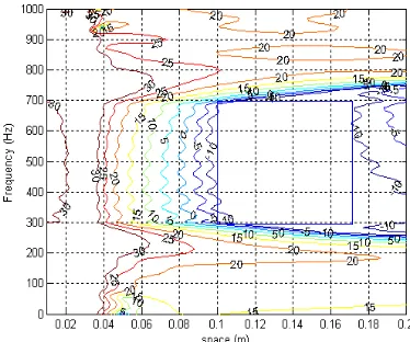
In the second example, constraints on amplification and robust stability are added to the optimization process to prevent a high amplification and instability. Equation (14) was used in the design process. Fig. 5 shows the attenuation contour over space and frequency with an amplification constraint not exceeding 20dB at the spatial axis from r=0.1m to r=0.2m for all frequencies and a constraint on robust stability with B1=B2=0.3. We can see that the attenuation area
becomes smaller than that without the amplification and robust stability constraints.
Fig. 7 shows the attenuation contour over space and frequency for three secondary monopoles with a constraint on robust stability for B1=B2=B3=0.3 and an amplification
constraint not to exceed 20dB at the spatial axis from r=0.1m to r=0.2m for all frequencies. It can be seen that the attenuation area becomes smaller than that without constraints on robust stability and amplification for three secondary monopoles.
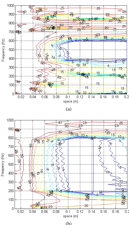
In the fifth example the effect of different minimization shapes on the size of the attenuation contours for three secondary monopoles has also been investigated in this study. Figs. 8 (a) and (b) show the attenuation contours over space and frequency for three secondary monopoles without constraints on robust stability and amplification for different minimization shapes. It can be seen that the shape of the 10dB attenuation contour changes with the minimization shape. In Fig. 8 (a) the 10dB attenuation contour has a narrow shape in frequency axis and longer in space axis similar to the minimization shape. When the minimization shape changes to be narrower in space axis and longer in frequency axis, the 10dB attenuation contour tends to extend its size in the frequency axis as shown in Fig. 8 (b). Therefore the shapes of the 10dB attenuation contour can be designed using the method presented in the paper.
V. CONCLUSIONS
The theory of active control for a broad-band diffuse field using two-channel and three-channel systems has been presented and the performance has been investigated through computer simulations. The acoustic pressure was minimized at the specified region over space and frequency. Constraints on amplification and robust stability were also included in the design process. The results showed that a good attenuation could be achieved at the desired range over space and frequency using a two-channel system. However, a better performance was achieved using a three-channel system. When limits on amplification and robust stability were introduced, the performance began to degrade. It has also been shown that acoustic pressure could be minimized at a specific frequency range and at a specific location in space away from the microphone. This could be realized by virtual microphone methods. Moreover, the shapes of the 10dB attenuation contour could be controlled using a three-channel system.
REFERENCES
[1] C. F. Ross, ‘‘Active control of sound’’, Dr. Thesis, University of Cambridge, U. K., 1980.
[2] P. Joseph, ‘‘Active control of high frequency enclosed sound fields’’, Dr. Thesis, University of Southampton, U. K., 1990. [3] P. A. Nelson and S. J. Elliott: Active Control of Sound , Academic, London, 1992.
[4] M. Miyoshi, J. Shimizu and N. Koizumi, ‘‘On arrangements of noise controlled points for producing larger quiet zones with multi-point active noise control’’, Inter-noise 94, 1994 p.1229. [5] J. Guo, J. Pan and C. Bao, ‘‘Avtively created quiet zones by multiple control sources in free space’’, J. Acoust. Soc. Am. 101, 1997 p.1492.
[6] W. K. Tseng, B. Rafaely, and S.J. Elliott, ‘‘2-norm and ∞-norm pressure minimisation for local active control of sound’’,
ACTIVE’99, 1999 p.661.
[7] W. K. Tseng, B. Rafaely, and S.J Elliott, ‘‘Local active sound control using 2-norm and ∞-norm pressure minimisation’’, Journal
of Sound and Vibration, 234(3) 2000 p.427.
[8] D. Halim and S. O. R. Moheimani, ‘‘Spatial H2 control of a piezoelectric laminate beam: experimental implementation’’, IEEE
Transactions on Control Systems Technology, 2002 Vol. 10, No.4
p.533.
[9] B. Rafaely, ‘‘Active control with optimisation over frequency and space’’, ACTIVE 99. 1999 p.1005.
[10] Wen-Kung Tseng,”Active noise control systems for broadband disturbance”, Jpn. Journal of Applied Physics, Vol.44, No. 5A, pp. 3165-3169 2005.
[11] Rafaely, B. "Spatial-temporal correlation of a diffuse sound field," Journal of the Acoustical Society of America, 107(6), 2000 p3254-3258.
[12] Chun, I., Rafaely, B. and Joseph, P., "Experimental investigation of spatial correlation of broadband diffuse sound fields," ," Journal of the Acoustical Society of America, 113(4), 2003 p1995-1998.
[13] Rafaely, B., "Zones of quiet in a broadband diffuse sound field," Journal of the Acoustical Society of America, 110(1), 2001 p296-302.
[14] Garcia-Bonito, J, Elliott, S.J. and Boucher, C.C.. ‘‘A novel secondary source for a local active noise control system’’. ACTIVE 97, 1997 p405-418.
[15] Jacobsen, F.. ‘‘The diffuse sound field’’. Report no. 27, The Acoustics Laboratory, Technical University of Denmark, 1979. [16] S. Skogestad and I. Postlethwaite: Multivariable Feedback
Control John Wiley & Sons, Chichester 1996.
[17] M. Morari, and E. Zafiriou: Robust Process Control
Prentice-Hall, NJ. 1989.
[18] G. F. Franklin, J. D. Powell, and A. Emamni-Naeini:
Feedback Control of Dynamic Systems Addison-Wesley, MA. 1994
controller
Primary field
Pressure minimization region
Desired zone of quiet
microphone Space﹝m﹞
monopoles S1 S2
C
o
n
tr
o
l ba
ndw
id
th
F
re
q
ue
ncy [
H
[image:5.595.66.264.68.206.2]z]
Figure 1. Configuration of acoustic pressure minimization over space and frequency with a two-channel feedback system.
C1
C2
Monopoles
S2 S1
Microphone
[image:5.595.312.495.71.214.2]Controllers
Figure 2. Two-channel feedback control system used to control broad-band disturbance.
PS2
PS1
+
+
_ _
_
+ + +
+ +
+
dS Disturbance away from microphone
es Error signal away from microphone d Disturbance at
microphone
e Error signal Control filter 1
Control filter 2
C1
C2
x
W2
W1 P1
P1o
P2
P2o
[image:5.595.313.497.274.417.2]Figure 3. Two-channel feedback control system with two internal model controllers.
Figure 4. Attenuation in decibels as function of space and frequency for two-channel system with two FIR filters having 64 coefficients without constraints.
Figure5. Attenuation in decibels as function of space and frequency for a two-channel system with two FIR filters having 64 coefficients and with constraints on amplification not exceeding 20dB at spatial axis from r=0.1m to r=0.2m for all frequencies and constraints on robust stability with B1 = B2
=0.3.
[image:5.595.55.258.482.672.2] [image:5.595.327.514.507.663.2]Figure 7. Attenuation in decibels as a function of space and frequency for a three-channel system with FIR filters having 64 coefficients and constraints on robust stability for B1=B2=B3=0.3 and amplification not to exceed 20dB at
the spatial axis from r=0.1m to r=0.2m for all the frequencies.
(a)
(b)
[image:6.595.59.265.320.678.2]