Abstract—Using multiple antennas at both sides of the wireless link is currently an active area of research because of the huge capacity and reliability gains promised by such systems. These gains are achieved almost for free where there is no extra bandwidth or transmit power is required. Such a system is called Multiple Input Multiple Output (MIMO) wireless system. In this paper, the behaviour of the MIMO Rayleigh channel’s eigenmodes and the power levels allocated to them by the water-filling algorithm with SNR and with the channel correlation will be analyzed. Capacity of the channel eigenmodes and total capacity of the channel will also be studied. It was found that, the strongest eigenmode of a channel matrix increases with correlation, while the other eigenmodes of the channel decrease. When the channel correlation approaches 1, the strongest eigenmode approaches the Mr * Mt, while the
other eigenmodes approach zero. At low SNR, to get the maximum capacity of the channel, the transmitter allocates all transmit power to the strongest eigenmode, and hence the channel capacity will be improved by the channel correlation. At high SNR, the transmitter divides this power equally among the eigenmodes to maximize the channel capacity. In this paper, the channel parameters are considered perfectly known at both sides of the wireless link.
Index Terms—Channel capacity, Channel correlation,
Channel eigenmodes, Low and high SNR.
I. INTRODUCTION
The field of wireless communications is rapidly evolving to achieve the increasing demands for high data rates and better quality of services [1]–[10]. These demands can be fulfilled using conventional systems, i.e. Single Input Single Output (SISO) -which are limited by multipath fading and interference- by increasing either the channel bandwidth, the transmit power, or both. However, this simplistic solution is not attractive for the following reasons. First, the transmit power can not exceed a certain value for its biological hazards, this is from one side. On the other side, building
Manuscript received December 18, 2008. This work was supported in part by the Malaysian Ministry of Science, Technology and Innovation (MOSTI) under the grant (01-01-02-SF0376).
A. Saad is with the Department of Electrical, Electronics and Systems Engineering, Universiti Kebangsaan Malaysia, 43600, Bangi, Selangor, Malaysia (e-mail: [email protected]).
M. Ismail is with the Department of Electrical, Electronics and Systems Engineering, Universiti Kebangsaan Malaysia, 43600, Bangi, Selangor, Malaysia (e-mail: [email protected]).
N. Misran is the Department of Electrical, Electronics and Systems Engineering, Universiti Kebangsaan Malaysia, 43600, Bangi, Selangor, Malaysia (e-mail: [email protected])
linear receivers with sensitivity beyond 30-35 dB is technically difficult and costly [11]. Second, frequency spectrum is a scarce and expensive resource especially below the 6 GHz. This makes it very difficult and costly to increase the channel bandwidth [11]. For these reasons, new techniques must be introduced to realize the needs of the modern wireless systems. These techniques must be affordable in terms of cost and biologically unharmful. Using multiple antennas at both sides of the wireless link, represents one of the most promising solutions to improve the bandwidth efficiency and system reliability without need to use extra bandwidth or transmitting more power into the channel [1], [2], [4]. Such a system is called Multiple Input Multiple Output (MIMO).
In MIMO systems, transmitter is equipped with more than one antenna to transmit the data and receiver is equipped with more than one antenna to receive this data. The capacities achieved by MIMO systems are very high comparing with the conventional systems (SISO, SIMO, and MISO). It has been proven that capacities of these systems increase linearly with the number of antenna pairs
if the channel is highly scattering and rich with multipath [1], [2].
These gains in capacity and reliability depend on the number of antennas at both sides, the statistics of the channel, and the channel knowledge at the transmitter [12].
Channel correlation is known to be one of the most undesired impairments that lead to MIMO channel capacity degradation [2], [13], [14], [15]. However, this is not always the case as we will see in this paper; where channel correlation is an advantage when the channel is known at the transmitter and when signal to noise ratio SNR is low. Channel correlation improves the channel capacity at low SNRs if the transmitter knows the channel matrix.
In this paper, the channel eigenmodes, the power allocated to them and the capacity of these eigenmodes will be studied and analyzed when the channel is known at the transmitter. This paper is organized as follows. In Section II, we will discuss the MIMO system model, the channel model and the correlation model used. MIMO channel capacity will be derived and developed in Section III. Section V is devoted to the simulation results and finally, the conclusions are drawn.
II. MIMO SYSTEM MODEL
Since MIMO is a narrowband technology [16], a narrowband, flat fading Rayleigh correlated channel and a single user, with Mt transmit and Mr receive antennas will be
Rayleigh Multiple Input Multiple Output (MIMO)
Channels: Eigenmodes and Capacity Evaluation
considered. The channel matrix H is assumed to be perfectly known at the receiver and the transmitter. The total transmit power from all antennas is Es, where Es is independent of the
number of antennas at the transmit side. This system is described as follows
y = Hx + n (1)
where x = [x1 x2…xMt]
T is the M
t × 1 complex vector
representing the transmitted signal with the power constraint tr (E (xxH))
≤
Es, (2)y = [y1 y2…yMr]Tis the Mr × 1 complex vector representing
the received signal and n = [n1 n2… nMr]Tis the Mr × 1
complex vector representing the additive white Gaussian noise vector (AWGN) with a zero mean and covariance matrix δ2
nIMr where IMr is the Mr × Mr identity matrix. (.)T,
(.)H, tr(.), and E(.) denote transposition, conjugate transpose,
trace, and expectation, respectively. H is the Mr × Mt MIMO
channel matrix, whose entries hij represent the complex
channel response of the channel between jthtransmit antenna
and the ith
receive antenna.
A. MIMO Channel Model
Kronecker model will be used here in this paper to describe the Rayleigh correlated channel. In this model the channel spatial correlation RH = E [vec (H) vec (HH)] [13],
where vec (H) denotes the MtMr × 1 vector formed by
stacking the columns of H. When the channel is rich with multipath and no LOS component exists, the transmit antennas correlation and receive antennas correlation can be considered independent. In such case, the channel correlation matrix RH can be decomposed into two correlation matrices,
the transmit correlation matrix Rt and the receive correlation
matrix Rr, so as RH = RtT
⊗
Rr, where⊗
is the Kroneckerproduct. Hence, the Rayleigh correlated channel can be written as H = Rr1/2 Hi.i.d Rt1/2, this channel model is called
Kronecker model. Where Rr is the receive correlation matrix,
and Rt is the transmit correlation matrix. Hi.i.d is the
uncorrelated white channel matrix. B. Correlation Model
The exponential correlation model will be adopted in this paper [17].
For this model, the components of the correlation matrices (Rrand Rt) are given by
rij =
1
,
,
≤
⎪⎩
⎪
⎨
⎧
>
≤
∗−
r
j
i
r
j
i
r
ji i j
where r is the complex correlation coefficient of neighboring antenna. This model is suitable for studying the effects of correlation on the channel capacity, although it is not accurate for some real world scenarios. However, this model is physically reasonable, where the correlation between the adjacent antennas is larger than the correlation between none-adjacent antennas [17].
III. MIMO CHANNEL CAPACITY
The theoretical capacity of this system is expressed by the following formula [1]
C = EH ⎥
⎦ ⎤ ⎢
⎣
⎡ +
) det(
log 2 H
M
M HQH
I
t r
ρ (3)
where, Q = E[xxH] is the input covariance matrix, and ρ
(SNR) = (Es/ N0), Es is the total transmit power, N0 is the
noise power in each antenna at the receive side.
In equation (3), the mean is taken over the random channel. The capacity depends on the number of antennas at both sides, input covariance matrix Q, and the channel statistics. When channel H is Rayleigh distributed, its mean will be zero (no LOS component exists) and its covariance is 1. Q represents the covariance matrix of the transmitted vector. This matrix is diagonal and its elements are all real numbers. The trace of this matrix should not exceed the number of transmit antennas. In other words, tr (Q) = Mt.
There are two cases for this matrix. When the transmitter does not have a prior knowledge about the channel matrix (i.e. uninformed transmitter), this matrix will be equal to the identity matrix Q =
t M
I
, meaning that the transmitter will divide the total transmitted power Es equally among itsantennas, and when the instantaneous channel matrix is available at the transmitter (informed transmitter), Q matrix can be optimized for optimum capacity. We will consider the latter case (Informed Transmitter case) in what follows,
A. Informed Transmitter
There is a possibility that transmitter learns the channel state information (CSI or channel matrix H) before it transmits the data vector. For instance, in TDD (Time Division Duplexing) systems, the channel matrix can be fed back to the transmitter from the receiver. In such an event, the capacity can be increased by resorting to the so-called waterfilling principle [18], by assigning various levels of transmit power to various transmitting antennas. This power is assigned on the bases that the better the channel is, the more power it gets and vice versa.
B. Waterfilling Algorithm
When H is known at the transmitter, waterfilling algorithm can be used to maximize the channel capacity by allocating more power to the eigenvalues that are in a good condition and less or none at all to the bad eigenvalues [18].
Given H = USVH (Singular Value Decomposition theorem or
SVD), the system expressed by equation (1) can be rewritten as
y = USVHx + n (4)
U is a matrix containing the eigenvectors of the receiver, V is a matrix containing the transmitter eigenvectors and the matrix S is a diagonal matrix containing the singular values (σi, where σi =
λ
i ) of the matrix H. U and V matrices are unitary, satisfying UUH= UHU = IMr, and VVH = VHV =
I
Mt. The transmitted vector is multiplied by a matrix V prior to transmission to cancel the effect of the matrix VH contained inH. In the same way, received vector is multiplied by a matrix UH to cancel the effect of the matrix U contained in H.
Substituting these values in equation (4), will produce the following
y’ = Sx’ + n’ (5) The system modeled by equation (5) is representing a group of parallel SISO channels; their power gains are the none zero diagonal elements of the matrix S.
The capacity of the MIMO channel is the sum of the individual parallel SISO channel capacities and is given by
⎥ ⎦ ⎤ ⎟⎟ ⎠ ⎞ ⎜⎜ ⎝ ⎛ + ⎢ ⎣ ⎡ =
∑
= t i
i rr i H M E
C log 1 ργ λ
1
2 (6) i
γ
is the amount of power transmitted over the eigenvalues iλ
such that∑
= = rr i t i M 1 γ and∑
= = rr i r ti M M
1
*
λ (7) Channel capacity maximization implies that transmitter accesses the individual sub-channels (the eigenvalues) and allocates variable power levels to them. Using Lagrangian method, the optimal energy allocated to each eigenvalue is
+ ⎟⎟ ⎠ ⎞ ⎜⎜ ⎝ ⎛ − = i t opt i M ρλ μ
γ ,i=1,2,…,rr (8) and
∑
= = rr i t opt i M 1γ (9) where,
μ
is a constant representing the water level and (x)+ implies(x)+= ⎩ ⎨ ⎧ ≥ 0 0 0 ≺ x if x if
x (10) Now, the optimal energy allocation is found iteratively through waterfilling algorithm as described below.
The iteration count p is set to 1, and then the constant
μ
in equation (8) is calculated based on the following formula,(
− +)
⎢⎣⎡ + ⎥⎦⎤ =∑
− + = 1 1 1 1 1 1 p rr i i t p rr M λ ρμ (11)
Using the obtained value of
μ
from equation (11), the power allocated to the ith eigenvalue can be calculated using⎟⎟ ⎠ ⎞ ⎜⎜ ⎝ ⎛ − = i t i M ρλ μ
γ , i= 1,2,…,rr– p+1. (12)
If the power allocated to the eigenvalue with the lowest gain is negative i.e. the term
i t
M
ρλ is greater than
μ
(the eigenvalue is bad), this eigenvalue is discarded and by setting0
1=
+ − opt p rrγ
and the algorithm is rerun with incrementing the iteration account by 1. This algorithm is repeated until all good eigenvalues are allocated the optimal power. The capacity of MIMO channels when the channel is known at the transmitter is at least equal to that obtained when thechannel is unknown at the transmitter. Once the optimal power allocation across the spatial eigenvalues is determined, the optimized input covariance matrix Q is now obtained,
Qopt=diag{ opt
rr opt opt
γ
γ
γ
1,
2,...,
} (13)and equation (3) will take the new form
C=EH ⎥
⎦ ⎤ ⎢ ⎣ ⎡ + ) det(
log2 opt H
M
M HQ H
I
t r
ρ (14)
At low SNR (ρ), waterfilling algorithm allocates all the available transmit power to the strongest eigenmode λmax (λmax = max (λi)). So equation (14) will reduce to the following equation at low SNR,
C
=
E
H[
log
2(
1
+
ρλ
max)
]
(15) Where ρ = Es/ N0 .When the channel H is orthogonal i.e. there is no correlation (unrealistic condition) all its eigenmodes (λi) will be equal (λi = 1, i = 1,2,3…min(Mt, Mr) ), so in this case there is no λmax since all the eigenmodes are equal and the condition number of the channel H is equal to 1 (λmax = λmin). However, Real channels are correlated, which means that the eigenmodes will not be equal and the condition number of the channel will not be equal to 1 (condition number of a channel H = λmax / λmin) because λmax will get larger and λmin will get smaller when the correlation increases. When channel correlation (r) approaches 1, λmax will approach Mr * Mt and all the other eigenmodes approaches zero. This means according to eq. (15) that capacity of the channel will increase when the channel correlation increases..
IV. SIMULATION RESULTS
In this paper, we study MIMO channel capacity over the SNR range from -20 dB to 20 dB, and channel correlation factor (r) takes the values from 0 to 0.9 at step 0.1. Channel matrix H is considered perfectly known at the transmitter and the receiver. Monte-Carlo simulation technique is used to estimate the channel capacity which is calculated at each SNR point by generating 10,000 channel matrices and taking the average over them.
equally among the channel eigenmodes. For this reason, the channel capacity at high SNRs is equal whether the channel matrix is known or unknown to the transmtter. Fig. 2 shows the power allocations for (3,3) channel.
-20 -10 0 10 20 30 40
0 0.2 0.4 0.6 0.8 1 1.2 1.4 1.6 1.8 2
SNR (dB) p
o we r l e ve l s
[image:4.595.302.540.58.219.2]gamma1 (2,4) gamma2 (2,4) gamma1 (2,10) gamma2 (2,10) gamma1 (2,2) gamma2 (2,2)
Fig.1: The power levels allocated to each eigenmode of a (2,2), (2,4) and (2,10) channels, r = 0.
-20 -10 0 10 20 30 40
0 0.5 1 1.5 2 2.5 3
SNR (dB) po
wer l ev el s
[image:4.595.44.289.106.244.2]gamma1 gamma2 gamma3
[image:4.595.44.287.107.427.2]Fig.2: The power levels allocated to each eigenmode of a (3,3) channel r = 0.
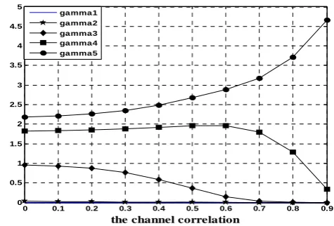
Fig. 3 and fig. 4 show the eigenmodes and the power levels allocated to them for a (5,5) channel. It is clear from fig. 4 that lambda5 increases when the channel correlation increases and the other eigenmodes of the channel decrease. When correlation approaches 1, the channel will have only one eigenmode which is lambda5 (lambda5 = 25, when correlation = 1) and all the other eigenmodes become zero.
0 0.1 0.2 0.3 0.4 0.5 0.6 0.7 0.8 0.9 0
5 10 15 20 25
the channel correlation t
h e c h a n n el ei g e n mo d es
lambda1 lambda2 lambda3 lambda4 lambda5
Fig.3: The (5,5) channel matrix eigenmodes at SNR = 0 dB.
0 0.1 0.2 0.3 0.4 0.5 0.6 0.7 0.8 0.9 0
0.5 1 1.5 2 2.5 3 3.5 4 4.5 5
the channel correlation t
he po
we
r l e v els
gamma1 gamma2 gamma3 gamma4 gamma5
Fig.4: The power levels allocated to each eigenmode of a (5,5) at SNR = 0 dB.
Fig. 5 and fig. 6 show the capacity of each eigenmode of a (2,2) channel in addition to the total capacity of the channel at (0, , 0.9) correlations. We can see that, when SNR is less than 0 dB the total capacity of the channel is equal to capacity of lambda2, and lambda1 is not contributing to the total capacity of the channel.
-200 -15 -10 -5 0 5 10 15 20 2
4 6 8 10 12 14
SNR (dB) c
ha n ne l c a pac it y
the capacity of lambda1 the capacity of lambda2 the total capacity
[image:4.595.309.548.335.492.2](cap. of lambda1+ cap. of lambda2)
Fig.5: The capacity of (2,2) channel, r = 0.
-20 -15 -10 -5 0 5 10 15 20
0 1 2 3 4 5 6 7 8 9
SNR (dB) c
h a n n el c a p a cit y
capacity of lambda1 capacity of lambda2 total capacity
(cap. of lambda1+cap. of lambda2)
Fig.6: the capacity of (2,2) channel, r = 0.9.
[image:4.595.37.280.550.701.2]-20 -15 -10 -5 0 5 10 15 20 0
5 10 15 20 25 30
SNR (dB) c
ha n ne l c a pac it y
Fig.7: The capacity of (5,5) channel, r = 0.
Finally, Fig. 9 shows how the capacity of a channel with Mt = 2, and Mr = 2,5,15 and at 0 dB change with the channel correlation. When Mr = 2, the capacity of the channel increases with the channel correlation because the (2,2) channel capacity at 0 dB depends only on lambda2, meaning that the total capacity of the channel is equal to the capacity produced by lambda2 (and the capacity of lambda1 is zero). We know from our discussion earlier that lambda2 of a (2,2) channel increases with the channel correlation, hence the capacity will also increase with channel correlation. When Mr = 15, the total capacity of the channel will be the summation of the capacity of lambda1 and the capacity of lambda2, hence the total capacity will decrease with the channel correlation.
-20 -15 -10 -5 0 5 10 15 20 0
2 4 6 8 10 12 14 16 18
SNR (dB) c
h a n n el c a p a cit y
cap. of lambda1 cap. of lambda2 cap. of lambda3 cap. of lambda4 cap. of lambda5 total capacity
Fig.8: The capacity of (5,5) channel, r = 0.9.
0 0.1 0.2 0.3 0.4 0.5 0.6 0.7 0.8 0.9 2
2.5 3 3.5 4 4.5 5 5.5 6 6.5
channel correlation c
h a n n el c a p a cit y
Mr = 2 Mr = 5 Mr = 15
Fig.9: the channel capacity of Mt = 2, Mr = 2,5,15 at SNR = 0dB.
V. CONCLUSION
In this paper, the eigenmodes of MIMO Rayleigh channels were studied and analyzed. First, the eigenmodes were evaluated how to change with SNR, and with the channel correlation. The power levels allocated to each eigenmode and how to change with SNR and channel correlation were also studied. The capacity of these eigenmodes was also evaluated. It was found that, the eigenmodes of any channel are independent of the SNRs, but depend on channel correlation. The maximum eigenmode of any MIMO channel increases with the channel correlation while all other eigenmodes decrease. When the channel correlation approaches 1, the maximum eigenmode approaches Mr * Mt, and all the other eigenmodes approach zero. Finally, when the SNR is low, the total capacity of the channel will be equal to the capacity of the largest eigenmode of this channel. Hence, the channel capacity will increase with the channel correlation.
REFERENCES
[1] I. E. Telatar, “Capacity of multi-antenna Gaussian channels,” European Transaction on Telecommunications, vol. 10, no. 6, pp. 585-595, Nov. 1999
[2] G. J. Foschini and M. J. Gans, “On limits of wireless communications in a fading environment when using multiple antennas,” Wireless Personal Communications, vol. 6, no. 3, pp. 311–335, Mar. 1998.
[3] G. G. Raleigh and J. M. Cioffi, “Spatio-temporal coding for wireless communication,” IEEE Trans. Commun., vol. 46, no. 3, pp. 357–366, Mar. 1998.
[4] G. J. Foschini, “Layered space-time architecture for wireless communication in a fading environment when using multi-element antennas,” Bell Labs. Tech. J., pp. 41–59, Autumn, 1996.
[5] V. Tarokh, N. Seshadri, and A. R. Calderbank, “Space-time codes for high data rate wireless communication: Performance criterion and code construction,” IEEE Trans. Inform. Theory, vol. 44, pp. 744–765, Mar. 1998.
[6] V. Tarokh, H. Jafarkhani, and A. R. Calderbank, “Space-time block codes from orthogonal designs,” IEEE Trans. Inform. Theory, vol. 45, pp. 1456–1467, July 1999.
[7] B. M. Hochwald and T. L. Marzetta, “Unitary space-time modulation for multiple-antenna communications in Rayleigh flat fading,” IEEE Trans.Inform. Theory, vol. 46, pp.
543–564, Mar. 2000.
[8] B. L. Hughes, “Differential space-time modulation,” IEEE Trans. Inform.Theory, vol. 46, pp. 2567–2578, Nov. 2000. [9] B. M. Hochwald, T. L. Marzetta, and B. Hassibi, “Space-time
autocoding,” IEEE Trans. Inform. Theory, vol. 47, pp. 2761–2781, Nov. 2001.
[10] A. Grant, “Rayleigh fading multiple-antenna channels,” EURASIP J .Appl. Signal Processing (Special Issue on Space-Time Coding (Part I)), vol. 2002, no. 3, pp. 316–329, Mar. 2002.
[11] A. J. Paulraj, D. Gore, R. U. Nabar, and H. Bolcskei “An overview of MIMO communications- a key to Gigabit wireless,” Proceeding of the IEEE, vol. 92, no. 2, Feb. 2004 [12] D. Gesbert, M. Shafi, D. Shiu, P. Smith, and A. Naguib, “From
theory to practice: an overview of MIMO space time coded wireless systems,” IEEE Journal on Selected Areas in Communications, vol. 21, no. 3, Apr. 2003
[14] S. L. Loyka, “Channel capacity of two-antenna BLAST architecture,” Electron. Lett., vol. 35, no. 17, pp. 1421–1422, Aug. 19, 1999.
[15] S. L. Loyka and J. R. Mosig, “Channel capacity of N-antenna BLAST architecture,” Electron. Lett., vol. 36, no. 7, pp. 660–661, Mar. 2000.
[16] S. Salous, The provision of an initial study of multiple in multiple out technology, available at
http://www.dur.ac.uk/comms.systems/summary2.pdf [17] S. Loyka, “Channel capacity of MIMO architecture using the
exponential correlation matrix,” IEEE Communications Letters, vol. 5, no. 9, Sep 2001.