Self-disclosure topic model for classifying and analyzing Twitter
conversations
JinYeong Bak∗
Department of Computer Science KAIST
Daejeon, South Korea
Chin-Yew Lin
Microsoft Research Beijing 100080, P.R. China
Alice Oh
Department of Computer Science KAIST
Daejeon, South Korea
Abstract
Self-disclosure, the act of revealing one-self to others, is an important social be-havior that strengthens interpersonal rela-tionships and increases social support. Al-though there are many social science stud-ies of self-disclosure, they are based on manual coding of small datasets and ques-tionnaires. We conduct a computational analysis of self-disclosure with a large dataset of naturally-occurring conversa-tions, a semi-supervised machine learning algorithm, and a computational analysis of the effects of self-disclosure on subse-quent conversations. We use a longitu-dinal dataset of 17 million tweets, all of which occurred in conversations that con-sist of five or more tweets directly reply-ing to the previous tweet, and from dyads with twenty of more conversations each. We develop self-disclosure topic model (SDTM), a variant of latent Dirichlet al-location (LDA) for automatically classi-fying the level of self-disclosure for each tweet. We take the results of SDTM and analyze the effects of self-disclosure on subsequent conversations. Our model sig-nificantly outperforms several comparable methods on classifying the level of self-disclosure, and the analysis of the longitu-dinal data using SDTM uncovers signifi-cant and positive correlation between self-disclosure and conversation frequency and length.
1 Introduction
Self-disclosure is an important and pervasive so-cial behavior. People disclose personal informa-tion about themselves to improve and maintain
∗This work was done when JinYeong Bak was a visiting student at Microsoft Research, Beijing, China.
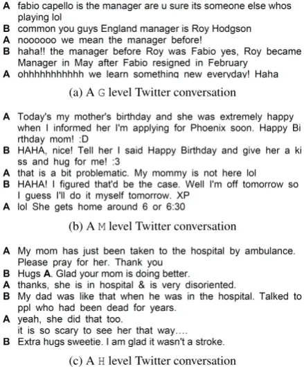
relationships (Jourard, 1971; Joinson and Paine, 2007). A common instance of self-disclosure is the start of a conversation with an exchange of names and additional self-introductions. Another example of self-disclosure, shown in Figure 1c, where the information disclosed about a family member’s serious illness, is much more personal than the exchange of names. In this paper, we seek to understand this important social behavior using a large-scale Twitter conversation data, automati-cally classifying the level of self-disclosure using machine learning and correlating the patterns with conversational behaviors which can serve as prox-ies for measuring intimacy between two conversa-tional partners.
Twitter conversation data, explained in more detail in section 4.1, enable an extremely large scale study of naturally-occurring self-disclosure behavior, compared to traditional social science studies. One challenge of such large scale study, though, remains in the lack of labeled ground-truth data of self-disclosure level. That is, naturally-occurring Twitter conversations do not come tagged with the level of self-disclosure in each conversation. To overcome that challenge, we propose a semi-supervised machine learning approach using probabilistic topic modeling. Our self-disclosure topic model (SDTM) assumes that self-disclosure behavior can be modeled using a combination of simple linguistic features (e.g., pronouns) with automatically discovered seman-tic themes (i.e., topics). For instance, an utterance “I am finally through with this disastrous relation-ship” uses a first-person pronoun and contains a topic about personal relationships.
In comparison with various other models, SDTM shows the highest accuracy, and the result-ing conversation frequency and length patterns on self-disclosure are shown different over time. Our contributions to the research community include the following:
• We present key features and prior knowl-edge for identifying self-disclosure level, and show relevance of it with experiment results (Sec. 2).
• We present a topic model that explicitly in-cludes the level of self-disclosure in a conver-sation using linguistic features and the latent semantic topics (Sec. 3).
• We collect a large dataset of Twitter conver-sations over three years and annotate a small subset with self-disclosure level (Sec. 4).
• We compare the classification accuracy of SDTM with other models and show that it performs the best (Sec. 5).
• We correlate the self-disclosure patterns and conversation behaviors to show that there is significant relationship over time (Sec. 6). 2 Self-Disclosure
In this section, we look at social science literature for definition of the levels of self-disclosure. Us-ing that definition, we devise an approach to au-tomatically identify the levels of self-disclosure in a large corpus of OSN conversations. We dis-cuss three approaches, first, using first-person pro-noun features, and second, extracting seed words and phrases from the Twitter conversation cor-pus, and third, extracting seed words and phrases from an external corpus of anonymously posted secrets, and we demonstrate the efficacy of those approaches with an annotated corpus.
2.1 Self-disclosure (SD) level
To analyze self-disclosure, researchers categorize self-disclosure language into three levels: G (gen-eral) for no disclosure, Mfor medium disclosure, and H for high disclosure (Vondracek and Von-dracek, 1971; Barak and Gluck-Ofri, 2007). Ut-terances that contain general (non-sensitive) in-formation about the self or someone close (e.g., a family member) are categorized as M. Exam-ples are personal events, past history, or future plans. Utterances about age, occupation and hob-bies are also included. Utterances that contain sensitive information about the self or someone close are categorized asH. Sensitive information includes personal characteristics, problematic be-haviors, physical appearance and wishful ideas. Generally, these are thoughts and information that
(a) AGlevel Twitter conversation
(b) AMlevel Twitter conversation
[image:2.595.306.526.63.328.2](c) AHlevel Twitter conversation
Figure 1: An example of a Twitter conversation (from annotated dataset) withG,MandHlevel of self-disclosure.
one would keep as secrets to himself. All other utterances, those that do not contain information about the self or someone close are categorized as G. Examples include gossip about celebrities or factual discourse about current events. Figure 1 shows Twitter conversation examples with G, M and H levels from annotated dataset (see Sec-tion 4.2 for a detailed descripSec-tion of the annotated dataset).
2.2 GLevel of Self-Disclosure
Category Words/Expressions
Unigram my, I, I’m, I’ll, but, was, I’ve, love, dad, have Bigram I love, I was, I have, my dad, go to, my mom,
with my, have to, to go, my mum
[image:3.595.304.535.62.136.2]Trigram I have a, is going to, to go to, want to go, and I was, going to miss, I love him, I think I, I was like, I wish I
Table 1: High ranked words and expressions by mutual information between G and M/H level in annotated conversations.
most highly ranked discriminative features contain a first-person pronoun.
2.3 MLevel of Self-Disclosure
Utterances with M level include two types: 1) information related with past events and future plans, and 2) general information about self (Barak and Gluck-Ofri, 2007). For the former, we add as seed trigrams ‘I have been’ and ‘I will’. For the latter, we use seven types of information generally accepted to be personally identifiable in-formation (McCallister, 2010), as listed in the left column of Table 2. To find the appropriate tri-grams for those, we take Twitter conversation data (described in Section 4.1) and look for trigrams that begin with ‘I’ and ‘my’ and occur more than 200 times. We then check each one to see whether it is related with any of the seven types listed in the table. As a result, we find 57 seed trigrams for Mlevel. Table 2 shows several examples.
Type Trigram
Name My name is, My last name Birthday My birthday is, My birthday party Location I live in, I lived in, I live on
Contact My email address, My phone number Occupation My job is, My new job
Education My high school, My college is Family My dad is, My mom is, My family is
Table 2: Example seed trigrams for identifyingM level ofSD. There are 51 of these used in SDTM.
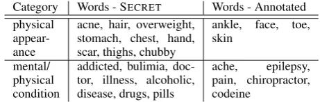
2.4 HLevel of Self-Disclosure
Utterances with H level express secretive wishes or sensitive information that exposes self or some-one close (Barak and Gluck-Ofri, 2007). These are generally kept as secrets. With this intuition, we crawled 26,523 posts fromSix Billion Secrets1
site where users post secrets anonymously2. We
1http://www.sixbillionsecrets.com 2This site is regularly monitored for spam.
Category Words - SECRET Words - Annotated physical
appear-ance
acne, hair, overweight, stomach, chest, hand, scar, thighs, chubby
ankle, face, toe, skin
mental/ physical condition
addicted, bulimia, doc-tor, illness, alcoholic, disease, drugs, pills
ache, epilepsy, pain, chiropractor, codeine
Table 3: Example words for identifyingHlevel of
SDfrom secret posts (2nd column) and annotated data (3rd column). Categories are hand-labeled.
call this external dataset SECRET. UnlikeGandM
levels, evidence ofHlevel of self-disclosure tends to be topical, such as physical appearance, mental and physical illnesses, and family problems, so we take an approach of fitting a topic model driven by seed words. A similar approach has been success-ful in sentiment classification (Jo and Oh, 2011; Kim et al., 2013).
A critical component of this approach is the set of seed words with which to drive the discovery of topics that are most indicative of Hlevel self-disclosure. To extract the seed words that express secretive personal information, we compute mu-tual information (Manning et al., 2008) with SE -CRET and 24,610 randomly selected tweets. We
select 1,000 words with high mutual information and filter out stop words. Table 3 shows some of these words. To extract seed trigrams of secretive wishes, we again look for trigrams that start with ‘I’ or ‘my’, occur more than 200 times, and select trigrams of wishful thinking, such as ‘I want to’, and ‘I wish I’. In total, there are 88 seed words and 8 seed trigrams forH.
Since SECRET is quite different from Twitter,
we must show that posts in SECRET are
seman-tically similar to theHlevel Tweets. Rather than directly comparing SECRETposts and Tweets, we
use the same method of extracting discriminative word features from the annotated H level Tweets (see Section 4.2). Table 3 shows the seed words extracted from SECRET as well as the annotated
Tweets. Because the annotated dataset consists of only 200 conversations, the coverage of the topics seems narrower than the much larger SECRETS,
but both datasets show similarities in the topics. This, combined with the results of the model with the two sets of seed words (see Section 5 for the results), shows that SECRETS is an effective and
𝑤 𝑧 𝜋
𝑟 𝛼 𝛾
C T N
𝑦
ω
𝜆 𝑥 𝜃𝑙
3
𝛽𝑙
𝜙𝑙
[image:4.595.102.262.62.180.2]𝐾𝑙 3
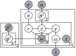
Figure 2: Graphical model of SDTM
Notation Description
G;M;H {general; medium; high}SDlevel
C;T;N Number of conversations; tweets; words
KG;KM;KH Number of topics for{G; M; H} c;ct Conversation; tweet in conversationc yct SDlevel of tweetct, G or M/H rct SDlevel of tweetct, M or H zct Topic of tweetct
wctn nthword in tweetct
λ Learned Maximum entropy parameters xct First-person pronouns features ωct Distribution overSDlevel of tweetct πc SDlevel proportion of conversationc θGc;θMc ;θHc Topic proportion of{G; M; H}in
con-versationc
φG;φM;φH Word distribution of{G; M; H} α;γ Dirichlet prior forθ;π βG,βM;βH Dirichlet prior forφG;φM;φH
ncl Number of tweets assignedSDlevell
in conversationc nl
ck Number of tweets assignedSDlevell
and topickin conversationc nl
kv Number of instances of wordvassigned SDlevelland topick
mctkv Number of instances of wordvassigned
[image:4.595.308.518.64.292.2]topickin tweetct
Table 4: Summary of notations used in SDTM
3 Self-Disclosure Topic Model
This section describes our model, the self-disclosure topic model (SDTM), for classifying self-disclosure level and discovering topics for each self-disclosure level.
3.1 Model
In section 2, we discussed different approaches to identifying each level of self-disclosure, based on social science literature, annotated and unan-notated Tweets, and an external corpus of se-cret posts. In this section, we describe our self-disclosure topic model, based on the widely used latent Dirichlet allocation (Blei et al., 2003), which incorporates those approaches.
Figure 2 illustrates the graphical model of
1. For each levell∈ {G,M,H}:
For each topick∈ {1, . . . , Kl}: Drawφlk∼Dir(βl) 2. For each conversationc∈ {1, . . . , C}:
(a) DrawθG
c ∼Dir(α) (b) DrawθM
c ∼Dir(α) (c) DrawθHc ∼Dir(α) (d) Drawπc∼Dir(γ)
(e) For each messaget∈ {1, . . . , T}:
i. Observe first-person pronouns featuresxct ii. Drawωct∼MaxEnt(xct,λ)
iii. Drawyct∼Bernoulli(ωct) iv. Ifyct= 0 which isGlevel:
A. Drawzct∼Mult(θGc) B. For each wordn∈ {1, . . . , N}:
Draw wordwctn∼Mult(φGzct)
Else which can beMorHlevel: A. Drawrct∼Mult(πc) B. Drawzct∼Mult(θrcct) C. For each wordn∈ {1, . . . , N}:
Draw wordwctn∼Mult(φrzctct) Figure 3: Generative process of SDTM.
SDTM and how those approaches are embodied in it. The first approach based on the first-person pronouns is implemented by the observed vari-able xct and the parameters λ from a maximum
entropy classifier for G vs. M/H level. The ap-proach of seed words and phrases for levelsMand His implemented by the three separate word-topic probability vectors for the three levels ofSD: φl
which has a Bayesian informative priorβlwhere
l∈ {G, M, H}, the three levels of self-disclosure. Table 4 lists the notations used in the model and the generative process, and Figure 3 describes the generative process.
3.2 ClassifyingGvsM/Hlevels
[image:4.595.73.294.206.497.2]3.3 ClassifyingMvsHlevels
The second part of the classification, theMand the Hlevel, is driven by informative priors with seed words and seed trigrams. In the graphical model,
r is the latent variable that represents this classi-fication, and π is the distribution over r. γ is a non-informative prior forπ, andβlis an informa-tive prior for eachSD level by seed words. For example, we assign a high value for the seed word ‘acne’ forβH, and a low value for ‘My name is’. This approach is the same as joint models of topic and sentiment (Jo and Oh, 2011; Kim et al., 2013).
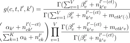
3.4 Inference
For posterior inference of SDTM, we use col-lapsed Gibbs sampling which integrates out la-tent random variables ω,π,θ, and φ. Then we only need to computey,randz for each tweet. We compute full conditional distributionp(yct =
j0, rct = l0, zct = k0|y
−ct,r−ct,z−ct,w,x) for
tweetctas follows:
p(yct = 0, zct=k0|y−ct,r−ct,z−ct,w,x)
∝ P1exp(λ0·xct)
j=0exp(λj ·xct) g(c, t, l
0, k0),
p(yct= 1, rct=l0, zct=k0|y−ct,r−ct,z−ct,w,x)
∝ P1exp(λ1·xct) j=0exp(λj·xct)(γl
0+n(−cl0ct))g(c, t, l0, k0),
wherez−ct,r−ct,y−ctarez,r,ywithout tweet
ct,mctk0(·)is the marginalized sum over wordvof mctk0v and the functiong(c, t, l0, k0)as follows:
g(c, t, l0, k0) = Γ(
PV
v=1βl
0
v +nl
0−(ct)
k0v )
Γ(PVv=1βl0
v +nl
0−(ct)
k0v +mctk0(·)) αk0 +nlck0(−0 ct)
PK
k=1αk+nlck0
! V
Y
v=1
Γ(βl0
v +nl
0−(ct)
k0v +mctk0v) Γ(βl0
v +nl
0−(ct)
k0v )
.
4 Data Collection and Annotation
To test our self-disclosure topic model, we use a large dataset of conversations consisting of Tweets over three years such that we can analyze the re-lationship between self-disclosure behavior and conversation frequency and length over time. We chose to crawl Twitter because it offers a prac-tical and large source of conversations (Ritter et al., 2010). Others have also analyzed Twitter con-versations for natural language and social media
[image:5.595.77.299.543.617.2]Users Dyads Conv’s Tweets 101,686 61,451 1,956,993 17,178,638
Table 5: Dataset of Twitter conversations. We chose conversations consisting of five or more tweets each. We chose dyads with twenty or more conversations.
research (boyd et al., 2010; Danescu-Niculescu-Mizil et al., 2011), but we collect conversations from the same set of dyads over several months for a unique longitudinal dataset. We also make sure that each conversation is at least five tweets, and that each dyad has at least twenty conversations.
4.1 Collecting Twitter conversations
We define a Twitter conversation as a chain of tweets where two users are consecutively reply-ing to each other’s tweets usreply-ing the Twitter reply button. We initialize the set of users by randomly sampling thirteen users who reply to other users in English from the Twitter public streams3. Then
we crawl each user’s public tweets, and look at users who are mentioned in those tweets. It is a breadth-first search in the network defined by users as nodes and edges as conversations. We run this search for dyads until the depth of four, and filter out users who tweet in a non-English language. We use an open source tool for de-tecting English tweets4. To protect users’ privacy,
we replace Twitter userid, usernames and url in tweets with random strings. This dataset consists of 101,686 users, 61,451 dyads, 1,956,993 conver-sations and 17,178,638 tweets which were posted between August 2007 to July 2013. Table 5 sum-marizes the dataset.
4.2 Annotating self-disclosure level
To measure the accuracy of our model, we ran-domly sample 301 conversations, each with ten or fewer tweets, and ask three judges, fluent in En-glish and graduate students/researchers, to anno-tate each tweet with the level of self-disclosure. Judges first read and discussed the definitions and examples of self-disclosure level shown in (Barak and Gluck-Ofri, 2007), then they worked sepa-rately on a Web-based platform.
As a result of annotation, there are 122Glevel converstaions, 147 M level and 32 H level
con-3https://dev.twitter.com/docs/api/
streaming
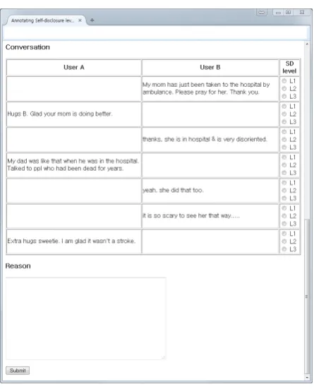
Figure 4: Screenshot of annotation web-based platform. Annotators read a Twitter conversation and annotate self-disclosure level to each tweet.
versations, and inter-rater agreement using Fleiss kappa (Fleiss, 1971) is 0.68, which is substantial agreement result (Landis and Koch, 1977).
5 Classification of Self-Disclosure Level This section describes experiments and results of SDTM as well as several other methods for classi-fication of self-disclosure level.
We first start with the annotated dataset in sec-tion 4.2 in which each tweet is annotated withSD
level. We then aggregate all of the tweets of a conversation, and we compute the proportions of tweets in eachSDlevel. When the proportion of tweets at M orH level is equal to or greater than 0.2, we take the level of the larger proportion and assign that level to the conversation. When the proportions of tweets atMorHlevel are both less than 0.2, we assignGto theSDlevel. The reason for setting 0.2 as the threshold is that a conversa-tion containing tweets with H orM level of self-disclosure usually starts with a greeting or a gen-eral comment, and contains one or more questions or comments before or after the self-disclosure tweet.
We compare SDTM with the following methods for classifying conversations forSDlevel:
• LDA (Blei et al., 2003): A Bayesian topic model. Each conversation is treated as a doc-ument. Used in previous work (Bak et al., 2012).
• MedLDA (Zhu et al., 2012): A super-vised topic model for document classifica-tion. Each conversation is treated as a doc-ument and response variable can be mapped to aSDlevel.
• LIWC (Tausczik and Pennebaker, 2010): Word counts of particular categories5. Used
in previous work (Houghton and Joinson, 2012).
• Bag of Words + Bigrams + Trigrams (BOW+): A bag of words, bigram and tri-gram features. We exclude features that ap-pear only once or twice.
• Seed words and trigrams (SEED): Occur-rences of seed words/trigrams from SECRET
which are described in section 3.3.
• SDTM with seed words from annotated Tweets (SDTM−): To compare with SDTM below using seed words from SECRET, this
uses seed words from the annotated data de-scribed in section 2.4.
• ASUM (Jo and Oh, 2011): A joint model of sentiments and topics. We map eachSD
level to one sentiment and use the same seed words/trigrams from SECRET as in SDTM
below. Used in previous work (Bak et al., 2012).
• First-person pronouns (FirstP): Occurrence of first-person pronouns which are described in section 3.2. To identify first-person pro-nouns, we tagged parts of speech in each tweet with the Twitter POS tagger (Owoputi et al., 2013).
• First-person pronouns + Seed words/trigrams (FP+SE1): First-person pronouns and seed words/trigrams from SECRET.
• Two stage classifier with First-person pro-nouns + Seed words/trigrams (FP+SE2): A
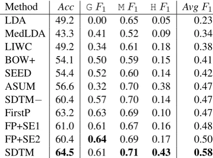
[image:6.595.72.295.57.333.2]Method Acc GF1 MF1 HF1 AvgF1 LDA 49.2 0.00 0.65 0.05 0.23 MedLDA 43.3 0.41 0.52 0.09 0.34 LIWC 49.2 0.34 0.61 0.18 0.38 BOW+ 54.1 0.50 0.59 0.15 0.41 SEED 54.4 0.52 0.60 0.14 0.42 ASUM 56.6 0.32 0.70 0.38 0.47 SDTM− 60.4 0.57 0.70 0.14 0.47 FirstP 63.2 0.63 0.69 0.10 0.47 FP+SE1 61.0 0.61 0.67 0.16 0.48 FP+SE2 60.4 0.64 0.69 0.17 0.50
[image:7.595.73.292.62.224.2]SDTM 64.5 0.61 0.71 0.43 0.58
Table 6:SDlevel classification accuracies and F-measures using annotated data. Acc is accuracy, andGF1 is F-measure for classifying theGlevel.
AvgF1 is the macroaveraged value ofGF1,MF1 andHF1. SDTM outperforms all other methods compared. The difference between SDTM and FirstP is statistically significant (p-value < 0.05
for accuracy,<0.0001forAvgF1).
two stage classifier with first-person pro-nouns and seed words/trigrams from SE -CRET. In the first stage, the classifier
identi-fiesGwith first-person pronouns. Then in the second stage, the classifier uses seed words and trigrams to identifyMandHlevels.
• SDTM: Our model with first-person pro-nouns and seed words/trigrams from SE -CRET.
SEED, LIWC, LDA and FirstP cannot be used directly for classification, so we use Maximum en-tropy model with outputs of each of those models as features6. BOW+ uses SVM with a radial
ba-sis kernel which performs better than all other set-tings tried including maximum entropy. We split the data randomly into 80/20 for train/test. We run MedLDA, ASUM and SDTM 20 times each and compute the average accuracies and F-measure for each level. We run LDA and MedLDA with var-ious number of topics from 80 to 140, and 120 topics shows best outputs. So we set 120 topics for LDA, MedLDA and ASUM, 60; 40; 40 topics for SDTMKG, KM andKH respectively which
is best perform from 40; 40; 40 to 60; 60; 60 top-ics. We assume that a conversation has few topics
6It performs better than other classifiers (C4.5, Naive-Bayes, SVM with linear kernel, polynomial kernel and radial basis)
and self-disclosure levels, so we setα =γ = 0.1
(Tang et al., 2014). To incorporate the seed words and trigrams into ASUM and SDTM, we initial-izeβG,βM andβH differently. We assign a high
value of 2.0 for each seed word and trigram for that level, and a low value of10−6 for each word that is a seed word for another level, and a default value of 0.01 for all other words. This approach is the same as previous papers (Jo and Oh, 2011; Kim et al., 2013).
As Table 6 shows, SDTM performs better than the other methods for accuracy as well as F-measure. LDA and MedLDA generally show the lowest performance, which is not surprising given these models are quite general and not tuned specifically for this type of semi-supervised clas-sification task. BOW which is simple word fea-tures also does not perform well, showing espe-cially low F-measure for theH level. LIWC and SEED perform better than LDA, but these have quite low F-measure for Gand Hlevels. ASUM shows better performance for classifying H level than others, confirming the effectiveness of a topic modeling approach to this difficult task, but not as well as SDTM. FirstP shows good F-measure for theGlevel, but theHlevel F-measure is quite low, even lower than SEED. Combining first-person pronouns and seed words and trigrams (FP+SE1) shows better than each feature alone, and the two stage classifier (FP+SE2) which is a similar ap-proach taken in SDTM shows better results. Fi-nally, SDTM classifiesG andMlevel at a similar accuracy with FirstP, FP+SE1 and FP+SE2, but it significantly improves accuracy for the Hlevel compared to all other methods.
6 Relations of Self-Disclosure and Conversation Behaviors
With SDTM, we can automatically classify the
SD level of a large number of conversations, so we investigate whether there is a similar relation-ship between self-disclosure in conversations and subsequent conversation behaviors with the same partner on Twitter.
For comparing conversation behaviors over time, we divided the conversations into two sets for each dyad. For theinitial period, we include conversations from the dyad’s first conversation to 20 days later. And for the subsequent period, we include conversations during the subsequent 10 days. We compute proportions of conversation for each SD level for each dyad in the initial and
subsequentperiods.
More specifically, we ask the following three questions:
1. If a dyad shows high conversation frequency at a particular time period, would they dis-play higher SDin their subsequent conver-sations?
2. If a dyad displays highSDlevel in their con-versations at a particular time period, would their subsequent conversations be longer?
3. If a dyad displays high overall SD level, would their conversations increase in length over time more than dyads with lower overall
SDlevel?
6.1 Experiment Setup
We first run SDTM with all of our Twitter con-versation data with 150; 120; 120 topics for SDTM KG, KM and KH respectively. The
hyper-parameters are the same as in section 5. To handle a large dataset, we employ a distributed al-gorithm (Newman et al., 2009), and run with 28 threads.
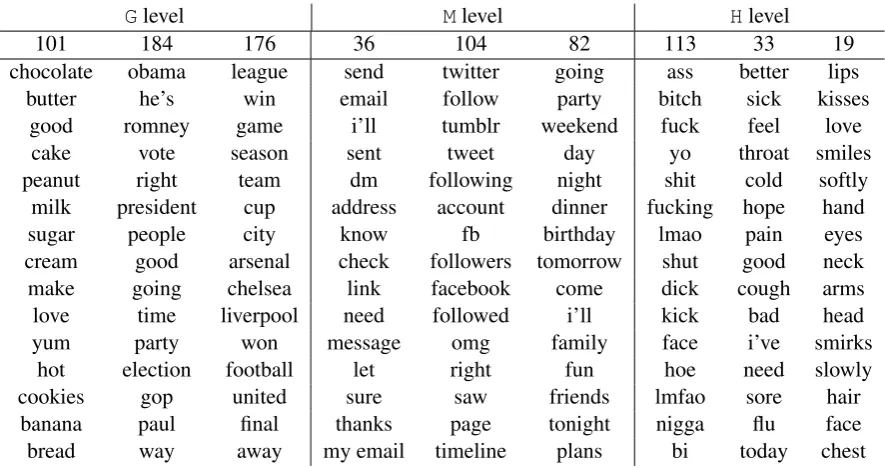
Table 7 shows some of the topics that were prominent in eachSDlevel by KL-divergence. As expected, Glevel includes general topics such as food, celebrity, soccer and IT devices,Mlevel in-cludes personal communication and birthday, and finally,Hlevel includes sickness and profanity.
We define a new measurement,SDlevel score for a dyad in the period, which is a weighted sum of each conversation withSDlevels mapped to 1, 2, and 3, for the levelsG,M, andH, respectively.
0 5 10 15 20 25 30 35
Initial conversation frequency 2.00
2.02 2.04 2.06 2.08 2.10 2.12 2.14
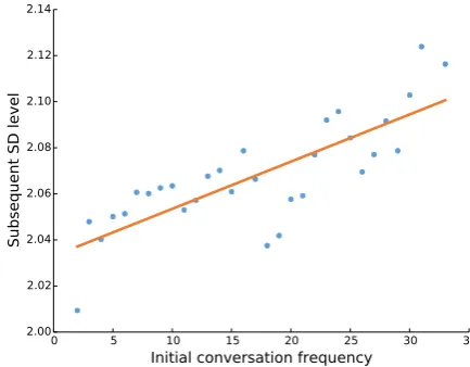
[image:8.595.307.524.64.233.2]Subsequent SD level
Figure 5: Relationship between initial conversa-tion frequency and subsequent SD level. The solid line is the linear regression line, and the co-efficient is0.0020withp <0.0001, which shows a significant positive relationship.
6.2 Does high frequency of conversation lead to more self-disclosure?
We investigate whether the initial conversation frequency is correlated with theSD level in the
subsequentperiod. We run linear regression with the initial conversation frequency as the indepen-dent variable, andSDlevel in the subsequent pe-riod as the dependent variable.
The regression coefficient is0.0020with low p-value (p < 0.0001). Figure 5 shows the scatter plot. We can see that the slope of the regression line is positive.
6.3 Does high self-disclosure lead to longer conversations?
Now we investigate the effect of the self-disclosure level to conversation length. We run linear regression with the intialSDlevel score as the independent variable, and the rate of change in conversation length between initial period andsubsequentperiod as the dependent variable. Conversation length is measured by the number of tweets in a conversation.
Glevel Mlevel Hlevel
101 184 176 36 104 82 113 33 19
chocolate obama league send twitter going ass better lips butter he’s win email follow party bitch sick kisses
good romney game i’ll tumblr weekend fuck feel love
cake vote season sent tweet day yo throat smiles
peanut right team dm following night shit cold softly milk president cup address account dinner fucking hope hand
sugar people city know fb birthday lmao pain eyes
cream good arsenal check followers tomorrow shut good neck make going chelsea link facebook come dick cough arms love time liverpool need followed i’ll kick bad head
yum party won message omg family face i’ve smirks
hot election football let right fun hoe need slowly cookies gop united sure saw friends lmfao sore hair
[image:9.595.78.521.61.295.2]banana paul final thanks page tonight nigga flu face bread way away my email timeline plans bi today chest
Table 7: High ranked topics in each level by comparing KL-divergence with other level’s topics
1.0 1.5 2.0 2.5 3.0
Initial SD level 0.10
0.05 0.00 0.05 0.10 0.15
[image:9.595.78.521.61.296.2]# Tweets in conversation changes proportion over time
Figure 6: Relationship between initial SD level and conversation length changes over time. The solid line is the linear regression line, and the co-efficient is 0.048 withp <0.0001, which shows a significant positive relationship.
6.4 Is there a difference in conversation length patterns over time depending on overall SD level?
Now we investigate the conversation length changes over time with three groups, low, medium, and high, by overall SD level. Then we investigate changes in conversation length over time.
Figure 7 shows the results of this investigation. First, conversations are generally lengthier when
SD level is high. This phenomenon is also
ob-0 5 10 15 20 25 30 35 40
Conversation order 8.0
8.5 9.0 9.5 10.0 10.5
# Tweets in conversation
high mid low
Figure 7: Changes in conversation length over time. We divide dyads into three groups by SD level score as low, medium, and high. Conversa-tion length noticeably increases over time in the medium and high groups, but only slight in the low group.
served in figure 6, but here we can see it as a long-term persistent pattern. Second, conversation length increases consistently and significantly for the high and medium groups, but for the lowSD
group, there is not a significant increase of conver-sation length over time.
7 Related Work
[image:9.595.308.525.336.504.2] [image:9.595.75.293.337.509.2]al., 2011; Trepte and Reinecke, 2013) or human annotation (Barak and Gluck-Ofri, 2007; Court-ney Walton and Rice, 2013). These methods con-sume much time and effort, so they are not suit-able for large-scale studies. In prior work clos-est to ours, Bak et al. (2012) showed that a topic model can be used to identify self-disclosure, but that work applies a two-step process in which a basic topic model is first applied to find the top-ics, and then the topics are post-processed for bi-nary classification of self-disclosure. We improve upon this work by applying a single unified model of topics and self-disclosure for high accuracy in classifying the three levels of self-disclosure.
Subjectivity which is aspect of expressing opin-ions (Pang and Lee, 2008; Wiebe et al., 2004) is related with self-disclosure, but they are different dimensions of linguistic behavior. Because there indeed are many high self-disclosure tweets that are subjective, but there are also counter examples in annotated dataset. The tweet “England manager is Roy Hodgson.” is low self-disclosure and low subjectivity, “I have barely any hair left.” is high self-disclosure but low subjectivity, and “Senator stop lying!” is low self-disclosure but high subjec-tivity.
8 Conclusion and Future Work
In this paper, we have presented the self-disclosure topic model (SDTM) for discovering topics and classifying SD levels from Twitter conversation data. We devised a set of effective seed words and trigrams, mined from a dataset of secrets. We also annotated Twitter conversations to make a ground-truth dataset for SD level. With anno-tated data, we showed that SDTM outperforms previous methods in classification accuracy and F-measure. We publish the source code of SDTM and the dataset include annotated Twitter conver-sations and SECRETpublicly7.
We also analyzed the relationship betweenSD
level and conversation behaviors over time. We found that there is a positive correlation be-tween initial SD level and subsequent conversa-tion length. Also, dyads show higher level of
SDif they initially display high conversation fre-quency. Finally, dyads with overall medium and highSDlevel will have longer conversations over time. These results support previous results in
so-7http://uilab.kaist.ac.kr/research/
EMNLP2014
cial psychology research with more robust results from a large-scale dataset, and show the effective-ness of computationally analyzing atSDbehavior. There are several future directions for this re-search. First, we can improve our modeling for higher accuracy and better interpretability. For instance, SDTM only considers first-person pro-nouns and topics. Naturally, there are other lin-guistic patterns that can be identified by humans but not captured by pronouns and topics. Sec-ond, the number of topics for each level is varied, and so we can explore nonparametric topic mod-els (Teh et al., 2006) which infer the number of topics from the data. Third, we can look at the relationship between self-disclosure behavior and general online social network usage beyond con-versations. We will explore these directions in our future work.
Acknowledgments
We would like to thank Jing Liu and Wayne Xin Zhao for inspiring discussions, and the anony-mous reviewers for helpful comments. Alice Oh is supported by ICT R&D program of MSIP/IITP [10041313, UX-oriented Mobile SW Platform].
References
JinYeong Bak, Suin Kim, and Alice Oh. 2012. Self-disclosure and relationship strength in twitter con-versations. InProceedings of ACL.
Azy Barak and Orit Gluck-Ofri. 2007. Degree and reciprocity of self-disclosure in online forums.
Cy-berPsychology & Behavior, 10(3):407–417.
David M Blei, Andrew Y Ng, and Michael I Jordan. 2003. Latent dirichlet allocation. Journal of
Ma-chine Learning Research, 3:993–1022.
danah boyd, Scott Golder, and Gilad Lotan. 2010. Tweet, tweet, retweet: Conversational aspects of retweeting on twitter. InProceedings of HICSS. S Courtney Walton and Ronald E Rice. 2013.
Medi-ated disclosure on twitter: The roles of gender and identity in boundary impermeability, valence, dis-closure, and stage. Computers in Human Behavior, 29(4):1465–1474.
Cristian Danescu-Niculescu-Mizil, Michael Gamon, and Susan Dumais. 2011. Mark my words!: Lin-guistic style accommodation in social media. In
Proceedings of WWW.
Tara M Emmers-Sommer. 2004. The effect of com-munication quality and quantity indicators on inti-macy and relational satisfaction. Journal of Social
Joseph L Fleiss. 1971. Measuring nominal scale agreement among many raters. Psychological
bul-letin, 76(5):378.
David J Houghton and Adam N Joinson. 2012. Linguistic markers of secrets and sensitive self-disclosure in twitter. InProceedings of HICSS. Yohan Jo and Alice H Oh. 2011. Aspect and
senti-ment unification model for online review analysis.
InProceedings of WSDM.
Adam N Joinson and Carina B Paine. 2007. Self-disclosure, privacy and the internet. The Oxford
handbook of Internet psychology, pages 237–252.
Adam N Joinson. 2001. Self-disclosure in computer-mediated communication: The role of self-awareness and visual anonymity. European
Journal of Social Psychology, 31(2):177–192.
Sidney M Jourard. 1971. Self-disclosure: An experi-mental analysis of the transparent self.
Suin Kim, Jianwen Zhang, Zheng Chen, Alice Oh, and Shixia Liu. 2013. A hierarchical aspect-sentiment model for online reviews. InProceedings of AAAI. J Richard Landis and Gary G Koch. 1977. The
mea-surement of observer agreement for categorical data.
biometrics, pages 159–174.
Andrew M Ledbetter, Joseph P Mazer, Jocelyn M DeG-root, Kevin R Meyer, Yuping Mao, and Brian Swaf-ford. 2011. Attitudes toward online social con-nection and self-disclosure as predictors of facebook communication and relational closeness.
Communi-cation Research, 38(1):27–53.
Christopher D Manning, Prabhakar Raghavan, and Hinrich Sch¨utze. 2008. Introduction to information
retrieval, volume 1. Cambridge University Press
Cambridge.
Erika McCallister. 2010. Guide to protecting the
confi-dentiality of personally identifiable information.
DI-ANE Publishing.
Arjun Mukherjee, Vivek Venkataraman, Bing Liu, and Sharon Meraz. 2013. Public dialogue: Analysis of tolerance in online discussions. InProceedings of
ACL.
David Newman, Arthur Asuncion, Padhraic Smyth, and Max Welling. 2009. Distributed algorithms for topic models. Journal of Machine Learning
Re-search, 10:1801–1828.
Olutobi Owoputi, Brendan OConnor, Chris Dyer, Kevin Gimpel, Nathan Schneider, and Noah A Smith. 2013. Improved part-of-speech tagging for online conversational text with word clusters. In
Proceedings of HLT-NAACL.
Bo Pang and Lillian Lee. 2008. Opinion mining and sentiment analysis. Found. Trends Inf. Retr., 2(1-2):1–135.
Alan Ritter, Colin Cherry, and Bill Dolan. 2010. Unsu-pervised modeling of twitter conversations. In
Pro-ceedings of HLT-NAACL.
Jian Tang, Zhaoshi Meng, Xuanlong Nguyen, Qiaozhu Mei, and Ming Zhang. 2014. Understanding the limiting factors of topic modeling via posterior con-traction analysis. In Proceedings of The 31st
In-ternational Conference on Machine Learning, pages
190–198.
Yla R Tausczik and James W Pennebaker. 2010. The psychological meaning of words: Liwc and comput-erized text analysis methods. Journal of Language
and Social Psychology.
Yee Whye Teh, Michael I Jordan, Matthew J Beal, and David M Blei. 2006. Hierarchical dirichlet pro-cesses. Journal of the american statistical
associ-ation, 101(476).
Sabine Trepte and Leonard Reinecke. 2013. The re-ciprocal effects of social network site use and the disposition for self-disclosure: A longitudinal study.
Computers in Human Behavior, 29(3):1102 – 1112.
Sarah I Vondracek and Fred W Vondracek. 1971. The manipulation and measurement of self-disclosure in preadolescents.Merrill-Palmer Quarterly of
Behav-ior and Development, 17(1):51–58.
Janyce Wiebe, Theresa Wilson, Rebecca Bruce, Matthew Bell, and Melanie Martin. 2004. Learn-ing subjective language. Computational linguistics, 30(3):277–308.
Wayne Xin Zhao, Jing Jiang, Hongfei Yan, and Xiaom-ing Li. 2010. Jointly modelXiaom-ing aspects and opin-ions with a maxent-lda hybrid. In Proceedings of
EMNLP.
Jun Zhu, Amr Ahmed, and Eric P Xing. 2012. Medlda: maximum margin supervised topic models. Journal