Neural Text Normalization with Subword Units

190

Neural Text Normalization with Subword Units

Courtney Mansfield†, Ming Sun‡, Yuzong Liu?, Ankur Gandhe?, Bj¨orn Hoffmeister?

†University of Washington, Seattle, WA, USA

[email protected]

‡Amazon Alexa AI, Seattle, WA, USA

[email protected]

?Amazon Alexa Speech, Seattle, WA, USA

{liuyuzon,aggandhe,bjornh}@amazon.com

Abstract

Text normalization (TN) is an important step in conversational systems. It converts writ-ten text to its spoken form to facilitate speech recognition, natural language understanding and text-to-speech synthesis. Finite state transducers (FSTs) are commonly used to build grammars that handle text normalization (Sproat,1996;Roark et al.,2012). However, translating linguistic knowledge into gram-mars requires extensive effort. In this paper, we frame TN as a machine translation task and tackle it with sequence-to-sequence (seq2seq) models. Previous research focuses on normal-izing a word (or phrase) with the help of lim-ited word-level context, while our approach directly normalizes full sentences. We find subword models with additional linguistic fea-tures yield the best performance (with a word error rate of0.17%).

1 Introduction

Non-standard words (NSWs) include expressions such as time or date (e.g., 4:58AM, 08-02, 8/2/2018), abbreviations (e.g., ft.) and letter se-quences (e.g., IBM, DL) (Sproat et al., 2001). They commonly appear in written texts such as websites, books and movie scripts. Writ-ten form of non-standard words can be normal-ized/verbalized to a spoken form, e.g., “August second”.

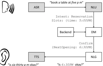
Although there is no incentive for human users to transcribe NSWs into spoken form, it plays an integral role in spoken dialog systems. As shown in Figure1, automatic speech recognition (ASR), natural language understanding (NLU) and text-to-speech synthesis (TTS) components all involve written-to-spoken form normalization or its in-verse process, spoken-to-written text normaliza-tion (ITN). ASR normalizes the training corpus before building its language model. Among many

benefits, such a model can reduce the size of the required vocabulary and address data sparsity is-sues. NLU might adopt ITN to recover the written text from ASR in run-time (e.g., “five p m ” →

“5:00PM”). In text-to-speech synthesis, for exam-ple, in order to pronounce “221B Baker St”, TTS needs to first convert the text to “two twenty one b baker street” and then generate the audio signal.

ASR NLU

DM

NLG TTS

“book a table atfive p m”

Intent: Reservation Slots: {time: 5:00PM}

Confirm {NextOpening: 6:30PM}

“Is 6:30PM okay?” “is six thirty p m okay?”

Backend

Figure 1: Text normalization in spoken dialog systems. Grey boxes involve text normalization or inverse text normalization.

Normalizing the written form text to its spoken form is difficult due to the following bottlenecks:

1. Lack of supervision — there is no incen-tive for people to produce spoken form text. Thus, it is hard to obtain a supervised dataset for training machine learning models;

2. Ambiguity — for written text, a change in context may require a different normaliza-tion. For example, “2/3” can be verbalized as a date or fraction depending on the meaning of the sentence.

as integer grammars (e.g., “26”→ “twenty six”) or time grammars (e.g., “5:26” → “five twenty six”). Constructing such grammars is time con-suming and error-prone and requires extensive lin-guistic knowledge and programming proficiency. Recently, with the rise of machine learning and es-pecially deep learning techniques, researchers are starting to bring more data-driven approaches to this field (Sproat and Jaitly,2016).

In this paper, we present our approach to non-standard text normalization via machine transla-tion techniques, where the source and target are written and spoken form text, respectively.

2 Related work

2.1 Finite state transducer

Normalizing written-form text to its spoken form has been approached by authoring weighted finite state transducer (WFST) grammars to handle in-dividual categories of NSW (e.g., time, date) and subsequently join them together (Sproat, 1996; Roark et al., 2012). One bottleneck to this ap-proach is the heavy demand of translating linguis-tic knowledge into WFSTs. A second problem is a lack of context awareness. For example, “dr.” may refer to “doctor” or “drive” in different con-texts. We have observed accuracy improvements by using an n-gram LM to re-rank hypotheses gen-erated by WFSTs. However, an n-gram LM’s con-text awareness is limited.

2.2 Data-driven approaches

Recently, methods based on neural networks have been applied to TN and ITN (Sproat and Jaitly, 2016; Pusateri et al., 2017; Yolchuyeva et al., 2018). To overcome one of the biggest problems — a lack of supervision, WFSTs have been used to transform large amounts of written-form text to its spoken form. Researchers hope a vast amount of such data can counteract the errors inherited in WFST-based models.

Recent data-driven approaches examine window-based sequence-to-sequence (seq2seq) models and convolutional neural networks (CNN) to normalize a central piece of text with the help of context (Sproat and Jaitly, 2016; Yolchuyeva et al., 2018). Window-based methods have the advantage of limiting the output vocabulary size, as most tokens that do not need to be transformed are labeled with a special<self>token.

Hybrid neural/WFST models have also been

proposed and applied to the text normalization problem (Pusateri et al., 2017;Yolchuyeva et al., 2018). Tokens in the input are first tagged with labels using machine learned models whereupon a handcrafted grammar corresponding to each la-bel conducts conversion. In both methods, a tag-ger is needed to first segment/label the input to-kens and conversion must be applied to each seg-ment to normalize a full sentence. Our seq2seq model does not require the aforementioned tagger (although could benefit from the tagger as we will show later) and directly translates a written-form sentence to its spoken form without grammars.

3 Model

3.1 Baseline models

Following Sproat and Jaitly (2016), we imple-ment a seq2seq model trained on window-based data. Table1illustrates the window-based model’s training examples corresponding to one sentence “wake me up at 8 AM .” which is broken down into 6 pairs. <n> and</n> indicate the center of the window. A window center might contain 1 or more words (e.g., “8 AM”) and the group-ing is provided by the dataset where each input sentence is segmented into chunks corresponding to labels such asTIME,DATE,ORDINAL(Sproat and Jaitly,2016). The model outputs tokens which correspond to the center of the window.

Table 1: In the window-based configuration,<n>and

</n>denote the center of the window. <self> indi-cates transforming the central piece to itself. This ex-ample illustrates a window size of 1.

Input Output

<n>wake</n>me <self> wake<n>me</n>up <self> me<n>up</n>at <self> up<n>at</n>8AM <self> at<n>8 AM</n>. eight a m AM<n>.</n> <sil>

level decoder.

A window-based seq2seq model, although able to attend well to a central piece of text, is not prac-tical for applying over a whole sentence. To ex-tend the model to full sentences, we break source sentences into segments. We then apply the model to one segment after another and concatenate their output tokens to produce full sentences.

As our second baseline, a seq2seq model is trained with full sentence data. As a result, it does not require any pre-processing step to gen-erate windows of text. It directly translates a sen-tence to its spoken form. Again, the encoder works at the character level while the decoder output se-quences of words while attention is used to align the input and output sequences.

3.2 Proposed model

There are several issues with the baseline seq2seq models. First of all, although there is no out-of-vocabulary (OOV) problem on the input side since it is modeled as a sequence of characters, the de-coder has an OOV issue–we cannot model every possible token. The window-based seq2seq adopts a special output token<self>that significantly re-duces the output vocabulary size. This is not prac-tical in the full sentence baseline as it requires the additional step of mapping each<self>in the out-put to a word in the inout-put.

Subwords have been shown to work well in open-vocabulary speech recognition and machine translation tasks (Sennrich et al.,2015;Qin et al., 2011). Subwords (i.e., a grouping of one or more characters) capture frequently co-occurring character combinations. For example, the word “subword” might be decomposed into two parts: “ sub” and “word”, where “ ” indicates the start of a word. An extreme case of the subword model is a character model. Compared with only characters, we believe segmenting input/output into subwords eases a seq2seq model’s burden of modeling long-distance dependencies.

3.2.1 Linguistic features

Sennrich and Haddow (2016) have shown that the addition of linguistic features can improve the quality of neural machine translation models. We observe that features such as casing and part-of-speech tags can also provide helpful insights into how a NSW should be normalized. For example, “US” should be normalized to “u s” instead of “us”. Similarly, part-of-speech tags can help the

model decide how to verbalize ambiguous forms such as “resume”, which is kept as-is as a verb or read out as “r´esum´e” as a noun. In regards to sub-words, it is important to know where the fragment comes from — beginning, middle, end of a word or the full word. For example, “id” should be nor-malized as “id” if it comes from the beginning of a word like “idea”. However, it could also be ver-balized as “i d” when taken as a standalone word.

In this paper, we explore linguistic features that are inexpensive to compute such as casing, POS, and positional features. We also use the edit la-bels from Google’s dataset (e.g.,TIME,DATE) al-though we acknowledge these labels are expensive and often times not accessible.

4 Experiments and results

4.1 Dataset

The data for the window-based seq2seq model and full sentence seq2seq were generated from the publicly available release of parallel writ-ten/speech formatted text from Sproat and Jaitly (2016). The set consists of Wikipedia text which was processed through Google TTS’s Kestrel text normalization system relying primarily on hand-crafted rules to produce speech-formatted text.

Although a large parallel dataset is available for English, we consider the feasibility of developing neural models for other languages which may not have text normalization systems in place. There-fore, we choose to scale the training data size to a limited set of text which could be generated by annotators in a reasonable time frame. As summa-rized in Table2, both window-based and sentence-based models are trained with 500K training in-stances.

Our datasets were randomly sampled from a set of 4.9M sentences in the training data portion of theSproat and Jaitly(2016) data release and split into training, validation, and test data. However, the training data for window-based and sentence-based models are not identical due to differences in input configurations. While the window-based model uses 500K randomly sampled windows, the sentence-based models use 500K sentences. For testing, 62.5K identical test sentences are used across all models. In order to decode sentences with the window-based model, sentences are first segmented into windows before inference.

Table 2: Size of training, validation, and test datasets. For the window-baseline, the data are pairs of win-dows and the normalization of the central piece of the window. For the sent-baseline and subword models, the data are pairs of sentences but in different formats — sent-baseline: (character sequence, word sequence); subword: (subword sequence, subword sequence). All models are evaluated on the same set of 62.5K sen-tences.

Model Train Valid Test Window-baseline 500K 62.4K 62.5K Sent-baseline 500K 62.5K 62.5K Subword 500K 62.5K 62.5K

ELECTRONICtext is not suitable for our system as it primarily reads out URLs letter by letter, e.g., “Forbes.com” → “f o r b e s dot c o m” (as opposed to “forbes dot com”). Therefore, we exclude ELECTRONIC data in our experiments. There are large numbers of<self>tokens present in the dataset. We followSproat and Jaitly(2016) in down-sampling window-based training data to constrain the proportion of “<self>” tokens to 10% of the data.

For training sentence-based models, the source sentence is segmented into characters while the target sentence is broken into tokens. For the sub-word model, both the source and target sentences are segmented into subword sequences. Subword units are concatenated to words for evaluation.

4.2 Baseline model setup

Our first approach replicates the window-based seq2seq model of Sproat and Jaitly (2016). The model encodes the central piece of text (1 or more tokens) including its context of N previous and following tokens at the character level. The out-put is a target token or a sequence of tokens. The input vocabulary consists of 250 common charac-ters including letcharac-ters, digits and symbols (e.g., $). The decoder vocabulary consists of 1K tokens in-cluding<self>and<sil>, the latter of which is used to normalize punctuation.

FollowingChan et al.(2016), we use a stacked (2-layer) bi-directional long short term memory network (bi-LSTM) as encoder and a stacked (2-layer) LSTM as decoder. We use 512 hidden states for the (bi-)LSTM. A softmax output distribution is computed over output vocabulary at each decod-ing step. Decoddecod-ing uses the attention mechanism fromBahdanau et al.(2014) and a beam size of 5.

Word and character embeddings are trained from scratch.

We use the OpenNMT toolkit (Klein et al., 2017) to train our models on a single P2.8xlarge Amazon EC2 instance. Models were trained with Stochastic Gradient Descent (SGD) on 200K timesteps (approximately 13 epochs). Approach-ing 200K timesteps, a significant decay in accu-racy and plateau in perplexity of the validation set occurred for all models. Validation occurred every 10K timesteps and the number of timesteps was chosen based on maximum accuracy on the valida-tion data. The learning rate was tuned to 1.0 for the window-based model and 0.5 for sentence-based models to achieve optimal performance. Learning rate decayed at a rate of 0.5 if perplexity on the validation set did not decrease or after 50K steps. A dropout of 0.3 was used across all models.

Figure 2: Evaluation of the window-based model. Cat-egories are sorted by frequency. *TELEPHONEis not reported in Sproat and Jaitly(2016) but included in the dataset; ** we removedELECTRONICcategory.

As shown in Figure 2, our replicated window-based model achieves reasonable performance compared withSproat and Jaitly (2016), consid-ering our training set is much smaller. There are 16 different edit labels shown. Data with

TELEPHONElabels were not included in the ini-tial analysis ofSproat and Jaitly (2016), but were made available in the dataset release.

the model to learn and predict.

4.3 Subword inventory

A subword inventory can be populated by data-driven approaches such as Byte Pair Encoding (BPE) (Sennrich et al., 2015). Text is first split into character sequences and the most frequently co-occurring units are greedily merged into one subword unit. This procedure continues until the desired subword inventory size is reached. Here, we enforce that two units cannot be merged if they cross a word boundary.

Table 3: Performance of different subword inventory sizes on validation set.

Inventory size SER (%) WER (%)

16K 3.56 0.92

8K 3.49 0.92

4K 3.34 0.90

2K 3.20 0.87

1K 3.17 0.90

500 3.53 1.01

To avoid OOV words, we also populate the sub-word inventory with the 250 most common char-acters used in the baseline model and digits 0-9. In data preparation, we force the subword model to split digits into a single subword piece (e.g., “1234” → “ 1 2 3 4”), regardless of whether a certain combination of numbers co-occur fre-quently (e.g., “19”). Tokenizing digits is benefi-cial when interpreting large sequences of numbers where every digit must be read out (e.g., 1,342→

“one thousand three hundred and forty two”). In this work, we use the SentencePiece toolkit1 and vary the inventory size. One can imagine that a larger subword inventory may contain longer sub-word entries. For example, the sub-word “anthology” is split into “ an th ology” by a subword model of 2K size and “ anth ology” by a model of 8K size. Our experiments find that an inventory size between 1K and 2K yields the best WER and SER (see Table3). For the rest of the paper, we use 2K.

4.4 Overall performance

Table 4 summarizes the performance of each model. We report sentence-error-rate (SER), word-error-rate (WER), BLEU score (Papineni et al., 2002) and latency (millisecond per input

1_{https://github.com/google/}

sentencepiece

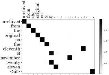
Figure 3: Attention visualization: x-axis is the input; y-axis is the output.

sentence), measured on the test set. We also re-port number of parameters and training time.

For the identity model, we replaced all non-alphanumerical characters in the source data with “<sil>”, except for spaces. As expected, this model generates a large number of errors. When evaluated on full sentences, the window-based model yields a reasonable accuracy, although it leverages a limited context. On the other hand, al-though the sentence baseline is directly trained on full sentences, its WER and SER are both worse than the window-based approach. The expan-sion of the output space significantly increases the trainable parameters from 10M to 55M, leading to more difficulties in training and inference.

As shown in Table 4, the subword model sig-nificantly outperforms baseline models in both ac-curacy and inference speed. Due to the source of the dataset (i.e., Wikipedia), test set and traing set have an overlap of about 27%. For in-stance, several source citations were commonly found in Wikipedia articles and appeared in train-ing and test (e.g., “IUCN Red List of Threatened Species.”). We found that, for sentences that were not seen by the subword model in training, our model still produces reliable outputs with a SER of4.59%and WER of1.09%.

Figure3 demonstrates that the attention mech-anism can effectively learn the non-monotonous nature of the text normalization problem as “eleventh”, “November” and “eleven” correspond to the third, second and first “11” in the input.

4.5 Linguistic features

We use the following linguistic features: 1)

Table 4: Comparison of models on test set.

Model SER WER BLEU Params Train Time Latency (%) (%) (M) (hours) (ms/sent)

Identity 99.39 32.70 51.74 N/A 0 N/A

Window-based 12.74 3.75 94.55 10 3.9 238 Sentence-based 48.67 9.26 82.28 55 8.0 159

Subword 3.31 0.91 98.79 12 10.0 88

Subword + Feat. w/o label 2.77 0.78 98.98 12 13.5 89 Subword + Feat. w/o casing 0.96 0.23 99.66 12 12.8 88 Subword + Feat. w/o POS 0.79 0.18 99.71 12 10.4 88 Subword + Feat. w/o position 0.80 0.17 99.73 12 13.0 88 Subword + All Feat. 0.78 0.17 99.73 12 15.4 89

beginning, middle, end, singleton; 3) POS tags: 44 Penn Treebank tags; 4)labels: 15 edit labels. Among these four types of features, capitalization and position are the least computationally expen-sive. POS tags are automatically predicted using an Averaged Perceptron Tagger from the Natural Language Toolkit (Bird et al., 2009). Edit labels are the most expensive to obtain in real life. Our labels are generated directly from the Google FST (Sproat and Jaitly,2016). Each type of feature is represented by a one-hot encoding.

To combine linguistic features with subword units, one can add or concatenate each subword’s embedding with its corresponding linguistic fea-ture embedding and feed a combined embedding to the bi-LSTM encoder. Or, a multi-layer percep-tron (MLP) can be applied to combine informa-tion in a non-linear way. Our experiments find that concatenation outperforms the other two methods. In Table 4we can see that the subword model with linguistic features produces the lowest SER (0.78%) and WER (0.17%). In addition, results from the ablation study show that each feature makes a positive contribution to the model. How-ever, edit labels seem to make the strongest contri-bution. We acknowledge that edit labels may not always be readily available. The model which uti-lizes all linguistic features except for edit labels still shows a16%relative SER reduction and14%

WER reduction over the subword model without linguistic features.

5 Discussion

Errors from the subword model are presented in Table5. Severe errors are shown in the first two rows. While these types of errors are infrequent, they change or obscure the meaning of the

utter-ance for a user. For example, the currency “nok” (e.g., “norwegian kroner”) was verbalized as “eu-ros”, reflecting a bias in the training data. While “euros” appeared 88 times, “norwegian kroner” appeared just 10 times.

Another type of error does not change the sen-tence meaning but can be unnatural. For example, “alexander iii” was predicted as “alexander three” rather than “alexander the third”. In this case, the referent of the sentence would likely be un-derstandable given context. Examples such as “5’ 11”” reflect the variety of natural readings which a human might produce. “Five foot eleven inches”, “five foot eleven”, and “five eleven” may all refer to a person’s height. Here the reference and model have produced different but acceptable variations.

Table 5: Errors from the subword model with linguistic features.

Input Reference Prediction

un u n un

nok 3 billion three billion three billion

norwegian kroner euros

alexander iii alexander the third alexander three

2000 gb two thousand two thousand

gigabytes g b

5’ 11” five foot eleven five eleven

a challenge for the academic community to come up with better data solutions.

6 Conclusion

In this paper, we investigate neural approaches to text normalization which directly translate a written-form sentence to its spoken counterpart without the need of a tagger or grammar. We show that the use of subwords can effectively reduce the OOV problem of a baseline seq2seq model with character inputs and token outputs. The addi-tion of linguistic features including casing, word position, POS tags, and edit labels leads to fur-ther gains. We empirically test the addition of each linguistic feature revealing that all features make a contribution to the model, and combin-ing features results in the best performance. Our model is an improvement over both window-based and sentence-based seq2seq baselines, yielding a WER of 0.17%.

References

Dzmitry Bahdanau, Kyunghyun Cho, and Yoshua Ben-gio. 2014. Neural machine translation by jointly learning to align and translate. arXiv preprint arXiv:1409.0473.

Steven Bird, Ewan Klein, and Edward Loper. 2009.

Natural language processing with Python: analyz-ing text with the natural language toolkit. ” O’Reilly Media, Inc.”.

William Chan, Navdeep Jaitly, Quoc Le, and Oriol Vinyals. 2016. Listen, attend and spell: A neural network for large vocabulary conversational speech recognition. In Acoustics, Speech and Signal Pro-cessing (ICASSP), 2016 IEEE International Confer-ence on, pages 4960–4964. IEEE.

Guillaume Klein, Yoon Kim, Yuntian Deng, Jean Senellart, and Alexander M Rush. 2017. OpenNMT: Open-source toolkit for neural machine translation.

arXiv preprint arXiv:1701.02810.

Kishore Papineni, Salim Roukos, Todd Ward, and Wei-Jing Zhu. 2002. Bleu: a method for automatic eval-uation of machine translation. In Proceedings of the 40th annual meeting on association for compu-tational linguistics, pages 311–318. Association for Computational Linguistics.

Ernest Pusateri, Bharat Ram Ambati, Elizabeth Brooks, Ondrej Platek, Donald McAllaster, and Venki Nagesha. 2017. A mostly data-driven ap-proach to inverse text normalization. Proc. Inter-speech 2017, pages 2784–2788.

Long Qin, Ming Sun, and Alexander Rudnicky. 2011. OOV detection and recovery using hybrid models with different fragments. In Twelfth Annual Con-ference of the International Speech Communication Association.

Brian Roark, Richard Sproat, Cyril Allauzen, Michael Riley, Jeffrey Sorensen, and Terry Tai. 2012. The openGrm open-source finite-state grammar software libraries. In Proceedings of the ACL 2012 System Demonstrations, pages 61–66. Association for Com-putational Linguistics.

Rico Sennrich and Barry Haddow. 2016. Linguistic input features improve neural machine translation.

arXiv preprint arXiv:1606.02892.

Rico Sennrich, Barry Haddow, and Alexandra Birch. 2015. Neural machine translation of rare words with subword units. arXiv preprint arXiv:1508.07909.

Richard Sproat. 1996. Multilingual text analysis for text-to-speech synthesis. Natural Language Engi-neering, 2(4):369–380.

Richard Sproat, Alan W. Black, Stanley Chen, Shankar Kumar, Mari Ostendorf, and Christopher Richards. 2001. Normalization of non-standard words. Com-puter Speech & Language, 15:287–333.

Richard Sproat and Navdeep Jaitly. 2016. RNN ap-proaches to text normalization: A challenge. arXiv preprint arXiv:1611.00068.