4187
What’s in a Name?
Reducing Bias in Bios without Access to Protected Attributes
Alexey Romanov1, Maria De-Arteaga2, Hanna Wallach3,
Jennifer Chayes3, Christian Borgs3, Alexandra Chouldechova2,
Sahin Geyik4, Krishnaram Kenthapadi4, Anna Rumshisky1, Adam Tauman Kalai3
1University of Massachusetts Lowell
{aromanov,arum}@cs.uml.edu
2Carnegie Mellon University
[email protected],[email protected]
3Microsoft Research
{wallach,jchayes,Christian.Borgs,Adam.Kalai}@microsoft.com
4LinkedIn
{sgeyik,kkenthapadi}@linkedin.com
Abstract
There is a growing body of work that proposes methods for mitigating bias in machine learn-ing systems. These methods typically rely on access to protected attributes such as race, gen-der, or age. However, this raises two signif-icant challenges: (1) protected attributes may not be available or it may not be legal to use them, and (2) it is often desirable to simulta-neously consider multiple protected attributes, as well as their intersections. In the context of mitigating bias in occupation classification, we propose a method for discouraging corre-lation between the predicted probability of an individual’s true occupation and a word em-bedding of their name. This method leverages the societal biases that are encoded in word embeddings, eliminating the need for access to protected attributes. Crucially, it only re-quires access to individuals’ names at training time and not at deployment time. We evaluate two variations of our proposed method using a large-scale dataset of online biographies. We find that both variations simultaneously reduce race and gender biases, with almost no reduc-tion in the classifier’s overall true positive rate.
1 Introduction
In recent years, the performance of machine learning systems has improved substantially, lead-ing to the widespread use of machine learnlead-ing
“What’s in a name? That which we call a rose by any other name would smell as sweet.” –William Shakespeare, Romeo and Juliet.
in many domains, including high-stakes domains such as healthcare, employment, and criminal jus-tice (Chalfin et al., 2016; Miotto et al., 2017; Chouldechova,2017). This increased prevalence has led many people to ask the question, “accurate, but for whom?” (Chouldechova and G’Sell,2017). When the performance of a machine learning system differs substantially for different groups of people, a number of concerns arise ( Baro-cas and Selbst, 2016; Kim, 2016). First and foremost, there is a risk that the deployment of such a method may harm already marginalized groups and widen existing inequalities. Recent work highlights this concern in the context of on-line recruiting and automated hiring (De-Arteaga et al., 2019). When predicting an individual’s occupation from their online biography, the au-thors show that if occupation-specific gender gaps in true positive rates are correlated with exist-ing gender imbalances in those occupations, then those imbalances will be compounded over time— a phenomenon sometimes referred to as the “leaky pipeline.” Second, the correlations that lead to per-formance differences between groups are often ir-relevant. For example, while an occupation clas-sifier should predict a higher probability of soft-ware engineer if an individual’s biography men-tions coding experience, there is no good reason for it to predict a lower probability of software en-gineer if the biography also mentions softball.
Some of the foundational papers in this area high-lighted the limitations of trying to mitigate bias using methods that are “unaware” of protected attributes such as race, gender, or age (e.g.,Dwork et al., 2012). As a result, subsequent work has primarily focused on introducing fairness con-straints, defined in terms of protected attributes, that reduce incentives to rely on undesirable correlations (e.g.,Hardt et al.,2016;Zhang et al., 2018). This approach is particularly useful if similar performance can be achieved by slightly different means—i.e., fairness constraints may aid in model selection if there are many near-optima.
In practice, though, any approach that relies on protected attributes may stand at odds with anti-discrimination law, which limits the use of pro-tected attributes in domains such as employment and education, even for the purpose of mitiging bias. And, in other domains, protected at-tributes are often not available (Holstein et al., 2019). Moreover, even when they are, it is usually desirable to simultaneously consider multiple pro-tected attributes, as well as their intersections. For example, Buolamwini (2017) showed that com-mercial gender classifiers have higher error rates for women with darker skin tones than for either women or people with darker skin tones overall.
We propose a method for reducing bias in machine learning classifiers without relying on protected attributes. In the context of occupation classification, this method discourages a classifier from learning a correlation between the predicted probability of an individual’s occupation and a word embedding of their name. Intuitively, the probability of an individual’s occupation should not depend on their name—nor on any protected attributes that may be inferred from it. We present two variations of our method—i.e., two loss func-tions that enforce this constraint—and show that they simultaneously reduce both race and gender biases with little reduction in classifier accuracy. Although we are motivated by the need to mitigate bias in online recruiting and automated hiring, our method can be applied in any domain where individuals’ names are available at training time.
Instead of relying on protected attributes, our method leverages the societal biases that are en-coded in word embeddings (Bolukbasi et al.,2016; Caliskan et al.,2017). In particular, we build on the work ofSwinger et al. (2019), which showed that word embeddings of names typically reflect
the societal biases that are associated with those names, including race, gender, and age biases, as well encoding information about other factors that influence naming practices such as national-ity and religion. By using word embeddings of names as a tool for mitigating bias, our method is conceptually simple and empirically powerful. Much like the “proxy fairness” approach ofGupta et al. (2018), it is applicable when protected at-tributes are not available; however, it additionally eliminates the need to specify which biases are to be mitigated, and allows simultaneous mitiga-tion of multiple biases, including those that re-late to group intersections. Moreover, our method only requires access to proxy information (i.e., names) at training time and not at deployment time, which avoids disparate treatment concerns and extends fairness gains to individuals with am-biguous names. For example, a method that ex-plicitly or imex-plicitly infers protected attributes from names at deployment time may fail to cor-rectly infer that an individual named Alex is fe-male and, in turn, fail to mitigate gender bias for her. Methodologically, our work is also similar to that ofZafar et al.(2017), which promotes fairness by requiring that the covariance between a pro-tected attribute and a data point’s distance from a classifier’s decision boundary is smaller than some constant. However, unlike our method, it requires access to protected attributes, and does not facili-tate simultaneous mitigation of multiple biases.
We present our method in Section 2. In sec-tion3, we describe our evaluation, followed by re-sults in Section4and conclusions in Section5.
2 Method
Our method discourages an occupation classifier from learning a correlation between the predicted probability of an individual’s occupation and a word embedding of their name. In this section, we present two variations of our method—i.e., two penalties that can be added to an arbitrary loss function and used when training any classifier.
clusters, it minimizes between-cluster disparities in the predicted probabilities of the true labels for the data points that correspond to the names in the clusters. In contrast, the second variation minimizes the covariance between the predicted probability of an individual’s occupation and a word embedding of their name. Because this variation minimizes the covariance directly, we call it Covariance Constrained Loss (CoCL). The most salient difference between these variations is that CluCL only minimizes disparities between the latent groups captured by the clusters. For example, if the clusters correspond only to gender, then CluCL is only capable of mitigating gender bias. However, given a sufficiently large number of clusters, CluCL is able to simultaneously mitigate multiple biases, including those that relate to group intersections. For both varia-tions, individual’s names are not used as input to the classifier itself; they appear only in the loss function used when training the classifier. The resulting trained classifier can therefore be deployed without access to individuals’ names.
2.1 Formulation
We definexi = {x1i, . . . , xMi }to be a data point,
yito be its corresponding (true) label, andnfi and
nlito be the first and last name of the correspond-ing individual. The classification task is then to (correctly) predict the label for each data point:
pi=H(xi) (1)
ˆ
yi= arg max
1≤j≤|C|
pi[j], (2)
whereH(·)is the classifier,Cis the set of possi-ble classes,pi ∈R|C|is the output of the classifier for data pointxi—e.g.,pi[j]is the predicted
prob-ability of xi belonging to class j—and yˆi is the
predicted label forxi. We definepyi to be the
pre-dicted probability ofyi—i.e., the true label forxi.
The conventional way to train such a classifier is to minimize some loss functionL, such as the cross-entropy loss function. Our method simply adds an additional penalty to this loss function:
Ltotal =L+λ· LCL, (3)
where LCL is either LCluCL orLCoCL (defined in Sections2.2and2.3, respectively), andλis a hy-perparameter that determines the strength of the penalty. This loss function is only used during training, and plays no role in the resulting trained
classifier. Moreover, it can be used in any standard setup for training a classifier—e.g., training a deep neural network using mini-batches and the Adam optimization algorithm (Kingma and Ba,2014).
2.2 Cluster Constrained Loss
This variation represents each first name nfi and last name nli as a pair of low-dimensional vec-tors using a set of pretrained word embeddingsE. These are then combined to form a single vector:
nei = 1 2
E[nfi] +E[nli]. (4)
Using k-means (Arthur and Vassilvitskii, 2007), CluCL then clusters the resulting embeddings into k clusters, yielding a cluster assignment ki for
each name (and corresponding data point). Next, for each classc∈C, CluCL computes the follow-ing average pairwise difference between clusters:
lc=
1
k(k−1)×
k
X
u,v=1
1
Nc,u
X
i:yi=c, ki=u
pyi − 1
Nc,v
X
i:yi=c, ki=v
pyi
2
,
(5)
whereuandvare clusters andNc,uis the number
of data points in clusterufor whichyi =c. CluCL
considers each class individually because different classes will likely have different numbers of train-ing data points and different disparities. Finally, CluCL computes the average ofl1, . . . l|C|to yield
LCluCL= 1
|C|
X
c∈C
lc. (6)
2.3 Covariance Constrained Loss
This variation minimizes the covariance between the predicted probability of a data point’s label and the corresponding individual’s name. Like CluCL, CoCL represents each name as a single vectornei and considers each class individually:
lc=Ei:yi=c
pyi −µcp
·(nei −µcn) , (7)
where µcp = Ei:yi=c[p y
i] andµcn = Ei:yi=c[n e i].
Finally, CoCL computes the following average:
LCoCL= 1
|C|
X
c∈C klck,
3 Evaluation
One of our method’s strengths is its ability to si-multaneously mitigate multiple biases without ac-cess to protected attributes; however, this strength also poses a challenge for evaluation. We are un-able to quantify this ability without access to these attributes. To facilitate evaluation, we focus on race and gender biases only because race and gen-der attributes are more readily available than at-tributes corresponding to other biases. We fur-ther conceptualize both race and gender to be bi-nary (“white/non-white” and “male/female”) but note that these conceptualizations are unrealistic, reductive simplifications that fail to capture many aspects of race and gender, and erase anyone who does not fit within their assumptions. We empha-size that we use race and gender attributes only for evaluation—they do not play a role in our method.
3.1 Datasets
We use two datasets to evaluate our method: the adult income dataset from the UCI Machine Learning Repository (Dheeru and Karra Taniski-dou, 2017), where the task is to predict whether an individual earns more than $50k per year (i.e., whether their occupation is “high status”), and a dataset of online biographies (De-Arteaga et al., 2019), where the task is to predict an individual’s occupation from the text of their online biography. Each data point in the Adult dataset consists of a set of binary, categorical, and continuous at-tributes, including race and gender. We prepro-cess these attributes to more easily allow us to understand the classifier’s decisions. Specifically, we normalize continuous attributes to be in the range [0,1] and we convert categorical attributes into binary indicator variables. Because the data points do not have names associated with them, we generate synthetic first names using the race and gender attributes. First, we use the dataset ofTzioumis(2018) to identify “white” and “non-white” names. For each name, if the proportion of “white” people with that name is higher than 0.5, we deem the name to be “white;” otherwise, we deem it to be “non-white.”1 Next, we use Social Security Administration data about baby names (2018) to identify “male” and “female” names. For each name, if the proportion of boys
1For 90% of the names, the proportion of “white” people
with that name is greater than 0.7 or less than 0.3, so there is a clear distinction between “white” and “non-white” names.
with that name is higher than 0.5, we deem the name to be “male;” otherwise, we deem it to be “female.”2 We then take the intersection of these two sets of names to yield a single set of names that is partitioned into four non-overlapping cat-egories by (binary) race and gender. Finally, we generate a synthetic first name for each data point by sampling a name from the relevant category.
Each data point in the Biosdataset consists of the text of an individual’s biography, written in the third person. We represent each biography as a vector of length V, where V is the size of the vocabulary. Each element corresponds to a single word type and is equal to 1 if the biog-raphy contains that type (and 0 otherwise). We limit the size of the vocabulary by discarding the 10% most common word types, as well as any word types that occur fewer than twenty times. Unlike the Adult dataset, each data point has a name associated with it. And, because biogra-phies are typically written in the third person and because pronouns are gendered in English, we can extract (likely) self-identified gender. We in-fer race for each data point by sampling from a Bernoulli distribution with probability equal to the average of the probability that an individual with that first name is “white” (from the dataset of Tzioumis(2018), using a threshold of 0.5, as described above) and the probability that an in-dividual with that last name is “white” (from the dataset ofComenetz (2016), also using a thresh-old of 0.5).3Finally, likeDe-Arteaga et al.(2019), we consider two versions of theBiosdataset: one where first names and pronouns are available to the classifier and one where they are “scrubbed.”
Throughout our evaluation, we use the fastText word embeddings, pretrained on Common Crawl data (Bojanowski et al.,2016), to represent names.
3.2 Classifier and Loss Function
Our method can be used with any classifier, including deep neural networks such as recur-rent neural networks and convolutional neural networks. However, because the focus of this paper is mitigating bias, not maximizing classifier
2For 98% of the names, the proportion of boys with that
name is greater than 0.7 or less than 0.3, so there is an even clearer distinction between “male” and “female” names.
3We note that, in general, an individual’s race or gender
accuracy, we use a single-layer neural network:
hi=Wh·xi+bh
pi=softmax(hi)
where Wh ∈ R|C|×M and bh ∈ R|C| are the weights. This structure allows us to examine indi-vidual elements of the matrixWh in order to
un-derstand the classifier’s decisions for any dataset. Both theAdultdataset and theBiosdataset have a strong class imbalance. We therefore use a weighted cross-entropy loss asL, with weights set to the values proposed byKing and Zeng(2001).
3.3 Quantifying Bias
To quantify race bias and gender bias, we fol-low the approach proposed by De-Arteaga et al. (2019) and compute the true positive rate (TPR) race gap and the TPR gender gap—i.e., the differ-ences in the TPRs between races and between gen-ders, respectively—for each occupation. The TPR race gap for occupationcis defined as follows:
TPRr,c =P
h
ˆ
Y =c|R=r, Y =ci (8)
Gapr,c =TPRr,c−TPR∼r,c, (9)
where r and ∼r are binary races, Yˆ and Y are random variables representing the predicted and true occupations for an individual, andRis a ran-dom variable representing that individual’s race. Similarly, the TPR gender gap for occupationcis
TPRg,c=P
h
ˆ
Y =c|G=g, Y =ci (10)
Gapg,c=TPRg,c−TPR∼g,c, (11)
wheregand∼gare binary genders andGis a ran-dom variable representing an individual’s gender.
To obtain a single score that quantifies race bias, thus facilitating comparisons, we calculate the root mean square of the per-occupation TPR race gaps:
GapRMSr =
s
1
|C|
X
c∈C
Gap2r,c. (12)
We obtain a single score that quantifies gender bias similarly. The motivation for using the root mean square instead of an average is that larger values have a larger effect and we are more interested in mitigating larger biases. Finally, to facilitate worst-case analyses, we calculate the maximum TPR race gap and the maximum TPR gender gap. We again emphasize that race and gender at-tributes are used only for evaluating our method.
4 Results
We first demonstrate that word embeddings of names encode information about race and gender. We then present the main results of our evaluation, before examining individual elements of the ma-trixWhin order to better understand our method.
4.1 Word Embeddings of Names as Proxies
We cluster the names associated with the data points in theBiosdataset, represented as word em-beddings, to verify that such embeddings indeed capture information about race and gender. We performk-means clustering (using thek-means++ algorithm) with k = 12 clusters, and then plot the number of data points in each cluster that correspond to each (inferred) race and gender. Fig-ures1aand1bdepict these numbers, respectively. Clusters 1, 2, 4, 7, 8, and 12 contain mostly “white” names, while clusters 3, 5, and 9 contain mostly “non-white names.” Similarly, clusters 4 and 8 contain mostly “female” names, while clus-ter 2 contains mostly “male” names. The other clusters are more balanced by race and gender. Manual inspection of the clusters reveals that clus-ter 9 contains mostly Asian names, while clusclus-ter 8 indeed contains mostly “female” names. The names in cluster 2 are mostly “white” and “male,” while the names in cluster 4 are mostly “white” and “female.” This suggests that the clusters are capturing at least some intersections. Together these results demonstrate that word embeddings of names do indeed encode at least some infor-mation about race and gender, even when first and last names are combined into a single embedding vector. For a longer discussion of the societal bi-ases reflected in word embeddings of names, we recommend the work ofSwinger et al.(2019).
4.2 AdultDataset
The results of our evaluation using the Adult
1 2 3 4 5 6 7 8 9 10 11 12
Cluster
0 10000 20000 30000 40000 50000 60000
Number of samples
White Not white Unknown
(a) Race.
1 2 3 4 5 6 7 8 9 10 11 12
Cluster
0 10000 20000 30000 40000 50000 60000
Number of samples
Female Male
[image:6.595.118.475.66.209.2](b) Gender.
Figure 1: Number of data points (from theBiosdataset) in each cluster that correspond to each race and gender.
Method λ Balanced TPR GapRMSg Gap
RMS
r Gap
max
g Gap
max
r
None 0 0.795 0.299 0.120 0.303 0.148
CluCL 1 0.788 0.278 0.121 0.297 0.145
CluCL 2 0.793 0.259 0.085 0.282 0.114
CoCL 1 0.794 0.215 0.091 0.251 0.119
[image:6.595.162.436.243.326.2]CoCL 2 0.790 0.163 0.080 0.201 0.109
Table 1: Results for theAdultdataset. Balanced TPR (i.e., per-occupation TPR, averaged over occupations), gender bias quantified as GapRMSg , race bias quantified as GapRMSr , maximum TPR gender gap, and maximum TPR race gap for different values of hyperparameterλ. Results are averaged over four runs with different random seeds.
0.0 0.1 0.2 0.3
RMS GAG
0.5 0.6 0.7 0.8
Accuracy Balanced
0.00 0.02 0.04 0.06 0.08 0.10 0.12
RMS RAG
GapRMSg GapRMSr
Balanced
TPR
Figure 2: Gender bias quantified as GapRMSg (left) and
race bias quantified as GapRMSr (right) versus balanced TPR for the CoCL variation of our method with dif-ferent values of hyperparameterλ(a larger dot means a larger value ofλ) for theAdult dataset. Results are averaged over four runs with different random seeds.
a less accurate classifier. Using λ = 0 leads to significant gender bias: the maximum TPR gen-der gap is 0.303. This means that the TPR is 30% higher for men than for women. We empha-size that this does not mean that the classifier is more likely to predict that a man earns more than $50k per year, but means that the classifier is more likely tocorrectly predict that a man earns more than $50k per year. Both variations of our method significantly reduce race and gender biases. With CluCL, the root mean square TPR race gap is re-duced from 0.12 to 0.085, while the root mean square TPR gender gap is reduced from 0.299 to
0.25. These reductions in bias result in less than one percent decrease in the balanced TPR (79.5% is decreased to 79.3%). With CoCL, the race and gender biases are further reduced: the root mean square TPR race gap is reduced to 0.08, while the root mean square TPR gender gap is reduced to 0.163, with 0.5% decrease in the balanced TPR.
[image:6.595.80.282.398.477.2]Method λ Balanced TPR GapRMSg Gap
RMS
r Gap
max
g Gap
max
r
None 0 0.788 0.173 0.051 0.511 0.121
CluCL 1 0.784 0.168 0.048 0.494 0.120
CluCL 2 0.781 0.165 0.047 0.486 0.114
CoCL 1 0.785 0.168 0.048 0.507 0.109
[image:7.595.163.437.64.147.2]CoCL 2 0.779 0.169 0.048 0.512 0.116
Table 2: Results for the originalBiosdataset. Balanced TPR (i.e., per-occupation TPR, averaged over occupations), gender bias quantified as GapRMSg , race bias quantified as GapRMSr , maximum TPR gender gap, and maximum TPR race gap for different values of hyperparameterλ. Results are averaged over four runs with different random seeds.
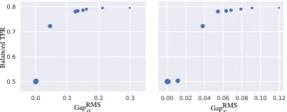
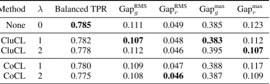
Method λ Balanced TPR GapRMSg GapRMSr Gapmaxg Gapmaxr
None 0 0.785 0.111 0.049 0.385 0.123
CluCL 1 0.782 0.107 0.048 0.383 0.112
CluCL 2 0.778 0.112 0.046 0.395 0.107
CoCL 1 0.780 0.109 0.047 0.388 0.117
CoCL 2 0.775 0.108 0.046 0.387 0.109
Table 3: Results for the “scrubbed”Biosdataset. Balanced TPR (i.e., per-occupation TPR, averaged over oc-cupations), gender bias quantified as GapRMSg , race bias quantified as GapRMSr , maximum TPR gender gap, and maximum TPR race gap for different values of hyperparameterλ. Again, results are averaged over four runs.
4.3 BiosDataset
The results of our evaluation using the original and “scrubbed” (i.e., names and pronouns are “scrubbed”) versions of theBiosdataset are shown in Tables2and3, respectively. The task is to pre-dict an individual’s occupation from the text of their online biography. Because the dataset has a strong class imbalance, we again report the bal-anced TPR. CluCL and CoCL reduce race and gender biases for both versions of the dataset. For the original version, CluCL reduces the root mean square TPR gender gap from 0.173 to 0.165 and the maximum TPR gender gap by 2.5%. Race bias is also reduced, though to a lesser extent. These reductions reduce the balanced TPR by 0.7%. For the “scrubbed” version, the reductions in race and gender biases are even smaller, likely because most of the information about race and gender has been removed by “scrubbing” names and pro-nouns. We hypothesize that these smaller reduc-tions in race and gender biases, compared to the
Adult dataset, are because the Adult dataset has fewer attributes and classes than theBiosdataset, and contains explicit race and gender information, making the task of reducing biases much sim-pler. We also note that each biography in the
Bios dataset is represented as a vector of length V, whereV is over 11,000. This means that the corresponding classifier has a very large number
of weights, and there is a strong overfitting effect. Because this overfitting effect increases withλ, we suspect it explains why CluCL has a larger root mean square TPR gender gap when λ = 2 than when λ = 1. Indeed, the root mean square TPR gender gap for the training set is 0.05 whenλ= 2. Using dropout and `2 weight regularization less-ened this effect, but did not eliminate it entirely.
4.4 Understanding the Method
Our method mitigates bias by making training-time adjustments to the classifier’s weights that minimize the correlation between the predicted probability of an individual’s occupation and a word embedding of their name. Because of our choice of classifier (a single-layer neural network, as described in Section3.2), we can examine in-dividual elements of the matrix Wh to
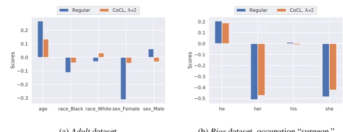
[image:7.595.166.435.205.289.2]age race_Black race_White sex_Female sex_Male 0.3
0.2 0.1 0.0 0.1 0.2
Scores
Regular CoCL, R=2λ=2
(a)Adultdataset.
he her his she
0.5 0.4 0.3 0.2 0.1 0.0 0.1 0.2
Scores
Regular CoCL, R=2λ=2
[image:8.595.117.468.68.203.2](b)Biosdataset, occupation “surgeon.”
Figure 3: Classifier weight values for several attributes for the conventional weighted cross-entropy loss function (i.e.,λ= 0) and for CoCL withλ= 2. Results are averaged over four runs with different random seeds.
the attribute “age” is also reduced, suggesting that CoCL may have mitigated some form of age bias. Figure3bdepicts the values of several weights specific to the occupation “surgeon” for the con-ventional weighted cross-entropy loss function (i.e., λ = 0) and for CoCL with λ = 2 for the original version of theBiosdataset. Whenλ= 0, the attributes “she” and “her” have large nega-tive weights, while the attribute “he” has a posi-tive weight. This means that the classifier is less likely to predict that a biography that contains the words “she” or “her” belongs to a surgeon. With CoCL, these magnitudes of these weights are re-duced, though these reductions are not as signifi-cant as the reductions shown for theAdultdataset.
5 Conclusion
In this paper, we propose a method for reducing bias in machine learning classifiers without rely-ing on protected attributes. In contrast to previous work, our method eliminates the need to specify which biases are to be mitigated, and allows si-multaneous mitigation of multiple biases, includ-ing those that relate to group intersections. Our method leverages the societal biases that are en-coded in word embeddings of names. Specifically, it discourages an occupation classifier from learn-ing a correlation between the predicted probability of an individual’s occupation and a word embed-ding of their name. We present two variations of our method, and evaluate them using a large-scale dataset of online biographies. We find that both variations simultaneously reduce race and gender biases, with almost no reduction in the classifier’s overall true positive rate. Our method is conceptu-ally simple and empiricconceptu-ally powerful, and can be used with any classifier, including deep neural
net-works. Finally, although we focus on English, we expect our method will work well for other lan-guages, but leave this direction for future work.
References
Social Security Administration. 2018. Baby names from social security card applications - national level data. Accessed 5 July 2018.
David Arthur and Sergei Vassilvitskii. 2007. k-means++: The advantages of careful seeding. In Proceedings of the eighteenth annual ACM-SIAM
symposium on Discrete algorithms, pages 1027–
1035. Society for Industrial and Applied Mathemat-ics.
Solon Barocas and Andrew D Selbst. 2016. Big data’s disparate impact. Cal. L. Rev., 104:671.
Piotr Bojanowski, Edouard Grave, Armand Joulin, and Tomas Mikolov. 2016. Enriching word vec-tors with subword information. arXiv preprint
arXiv:1607.04606.
Tolga Bolukbasi, Kai-Wei Chang, James Y Zou, Venkatesh Saligrama, and Adam T Kalai. 2016. Man is to computer programmer as woman is to homemaker? debiasing word embeddings. In
Ad-vances in Neural Information Processing Systems,
pages 4349–4357.
Joy Adowaa Buolamwini. 2017.Gender shades: inter-sectional phenotypic and demographic evaluation of
face datasets and gender classifiers. Ph.D. thesis,
Massachusetts Institute of Technology.
Aylin Caliskan, Joanna J Bryson, and Arvind Narayanan. 2017. Semantics derived automatically from language corpora contain human-like biases.
Science, 356(6334):183–186.
human capital with machine learning. American
Economic Review, 106(5):124–27.
Alexandra Chouldechova. 2017. Fair prediction with disparate impact: A study of bias in recidivism pre-diction instruments.Big data, 5(2):153–163.
Alexandra Chouldechova and Max G’Sell. 2017. Fairer and more accurate, but for whom? arXiv
preprint arXiv:1707.00046.
Joshua Comenetz. 2016. Frequently occurring sur-names in the 2010 census. United States Census
Bureau.
Maria De-Arteaga, Alexey Romanov, Hanna Wal-lach, Jennifer Chayes, Christian Borgs, Alexandra Chouldechova, Sahin Geyik, Krishnaram Kentha-padi, and Adam Tauman Kalai. 2019. Bias in bios: A case study of semantic representation bias in a high-stakes setting. InProceedings of the
Confer-ence on Fairness, Accountability, and Transparency,
pages 120–128. ACM.
Dua Dheeru and Efi Karra Taniskidou. 2017. UCI ma-chine learning repository.
Cynthia Dwork, Moritz Hardt, Toniann Pitassi, Omer Reingold, and Richard Zemel. 2012. Fairness through awareness. In Proceedings of the 3rd In-novations in Theoretical Computer Science Confer-ence, ITCS ’12, pages 214–226, New York, NY, USA. ACM.
Maya Gupta, Andrew Cotter, Mahdi Milani Fard, and Serena Wang. 2018. Proxy fairness. arXiv preprint
arXiv:1806.11212.
Moritz Hardt, Eric Price, Nati Srebro, et al. 2016. Equality of opportunity in supervised learning. In
Advances in neural information processing systems,
pages 3315–3323.
K. Holstein, J. Wortman Vaughan, H. Daum´e III, M. Dud´ık, and H. Wallach. 2019. Improving fair-ness in machine learning systems: What do industry practitioners need? InProceedings of the ACM CHI Conference on Human Factors in Computing
Sys-tems.
Pauline T Kim. 2016. Data-driven discrimination at work. Wm. & Mary L. Rev., 58:857.
Gary King and Langche Zeng. 2001. Logistic regres-sion in rare events data. Political Analysis, 9:137– 163.
Diederik P Kingma and Jimmy Ba. 2014. Adam: A method for stochastic optimization. arXiv preprint
arXiv:1412.6980.
Riccardo Miotto, Fei Wang, Shuang Wang, Xiaoqian Jiang, and Joel T Dudley. 2017. Deep learning for healthcare: review, opportunities and challenges.
Briefings in bioinformatics, 19(6):1236–1246.
Nathaniel Swinger, Maria De-Arteaga, IV Heffernan, Neil Thomas, Mark DM Leiserson, and Adam Tau-man Kalai. 2019. What are the biases in my word embedding? Proceedings of the 2019 AAAI/ACM
Conference on AI, Ethics, and Society.
Konstantinos Tzioumis. 2018. Demographic aspects of first names. Scientific data, 5:180025.
Muhammad Bilal Zafar, Isabel Valera, Manuel Gomez Rogriguez, and Krishna P Gummadi. 2017. Fairness constraints: Mechanisms for fair classification. In
Artificial Intelligence and Statistics, pages 962–970.
Brian Hu Zhang, Blake Lemoine, and Margaret Mitchell. 2018. Mitigating unwanted biases with adversarial learning. In Proceedings of the 2018
AAAI/ACM Conference on AI, Ethics, and Society,