HUMIR at IEST 2018: Lexicon Sensitive and Left Right Context Sensitive BiLSTM for Implicit Emotion Recognition

Proceedings of the 9th Workshop on Computational Approaches to Subjectivity, Sentiment and Social Media Analysis, pages 182–188 182

HUMIR at IEST-2018: Lexicon-Sensitive and Left-Right

Context-Sensitive BiLSTM for Implicit Emotion Recognition

Behzad Naderalvojoud, Alaettin Ucan and Ebru Akcapinar Sezer

Department of Computer Engineering Hacettepe University, Turkey

{n.behzad, aucan, ebru}@hacettepe.edu.tr

Abstract

This paper describes the approaches used in HUMIR system for the WASSA-2018 shared task on the implicit emotion recognition. The objective of this task is to predict the emotion expressed by the target word that has been ex-cluded from the given tweet. We suppose this task as a word sense disambiguation in which the target word is considered as a synthetic word that can express 6 emotions depending on the context. To predict the correct emo-tion, we propose a deep neural network model that uses two BiLSTM networks to represent the contexts in the left and right sides of the target word. The BiLSTM outputs achieved from the left and right contexts are consid-ered as context-sensitive features. These fea-tures are used in a feed-forward neural net-work to predict the target word emotion. Be-sides this approach, we also combine the BiL-STM model with lexicon-based and emotion-based features. Finally, we employ all mod-els in the final system using Bagging ensemble method. We achieved macro F-measure value of 68.8 on the official test set and ranked sixth out of 30 participants.

1 Introduction

Textual emotion recognition has received increas-ing attention in the natural language processincreas-ing and computational linguistics in the recent decade. It aims to identify the emotion expressed by the given text based on two emotion models: cat-egorical model and dimensional model (Russell 2003). While the categorical one uses discrete emotional categories such as Ekman’s six basic emotions (Ekman,1992), the dimensional one de-fines emotions in ak-dimensionalspace; each di-mension represents an attribute of the emotion such as valence, arousal and dominance. How-ever, the objective of the Implicit Emotion Shared Task (IEST) is to predict the emotion expressed

by the target word excluded from the given tweet instead of the emotion expressed by the tweet (Klinger et al.,2018). This task is organized based on the categorical model over 6 emotion categories asanger,disgust,fear,joy,sadness, andsurprise. Many approaches have been proposed for tex-tual emotion recognition task. In general, these approaches can be grouped into 3 main cate-gories: rule-based approaches, machine learning approaches and deep learning approaches. Rule based approaches exploit linguistic lexical re-sources like WordNet-Affect (Strapparava et al.,

2004) as well as unsupervised techniques such as Latent Semantic Analysis (LSA) in rule-based classifiers (Kim et al.,2010;Lee et al.,2010). The second group of the approaches employs machine learning algorithms –such as support vector ma-chines, naive Bayes, random forest, logistic re-gression, etc– to classify a text into emotion cat-egories (Liew and Turtle, 2016). This group of approaches needs an extensive feature engineering as well as domain knowledge. Furthermore, in this group, many of emotion lexicons which are gener-ated manually or automatically play an important role in extracting emotion-specific features. For instance, (Mohammad et al., 2013) proposes an SVM classifier based on a variety of feature sets extracted from manually and automatically gener-ated sentiment lexicons and (K¨oper et al., 2017) exploits several lexicon-based features and em-ploys them in the random forest classifier.

Unlike the previous approach, deep learning methods do not require any extensive feature en-gineering and can automatically extract features from raw text. Long Short-Term Memory (LSTM) and Convolutional Neural Network (CNN) are the basis of many approaches in deep learning for emotion recognition (Abdul-Mageed and Ungar,

to handle the semantic compositionality and to model the compositional changes on the text se-mantic according to its syntactic and sese-mantic structure. However, some methods train CNN and LSTM models jointly (Stojanovski et al., 2016) or use a CNN followed by a LSTM (Wang et al.,

2016;K¨oper et al.,2017).

In this paper, we suppose the target word as a synthetic ambiguous word that can express 6 emo-tions depending on the context. To predict the cor-rect emotion, we propose 7 deep neural network models that use three context-sensitive, lexicon-basedandemotion-weightfeatures. The influence of these features is investigated over the proposed deep neural network models where they are em-ployed to identify the context-dependent emotion of the target word.

2 System Description

In this section, we describe our proposed system to predict the emotion expressed by the target word which has been excluded from the tweet. In this system, we employ 6 deep neural network mod-els along with a multi-layer perceptron (MLP) and combine them into a single predictive model us-ing an ensemble method. All the models are ob-tained from 4 different approaches namely BiL-STM, Lexicon-BiLBiL-STM, Left-Right BilSTM and Lexicon-MLP. In these models, three kinds of fea-tures are extracted from a tweet and feed into a feed forward neural network: (1)context-sensitive features that are extracted from hidden state vec-tors of the BiLSTM network, (2) lexicon-based features that are obtained from AffectiveTweets Weka package (Mohammad and Bravo-Marquez,

2017) and (3) emotion-weight features that are computed by a feature evaluation metric proposed in (Naderalvojoud et al.,2015). In the following sections, we will describe our models and explain how they use these features to predict the emotion of the target word.

2.1 Feature Sets

The first feature set is obtained from the output of the Bidirectional Long Short-Term Memory (BiL-STM) network. BiLSTM is a variant of Recurrent Neural Network that uses LSTM cells to model a sequence. It encodes a tweet once from the be-ginning to end (left-to-right) and once from end to beginning (right-to-left). As a result, it maps a tweet to a pair of hidden state vectors. These

vectors are used as context-sensitive features in our system to learn the semantic composition ef-fects. The second kind of features are extracted from different sentiment and emotion lexicons. We have used 45 lexicon-based features extracted from the AffactiveTweet of Weka package. The details of these features can be found in ( Moham-mad and Bravo-Marquez, 2017). We also pro-pose 6 emotion-weight features (corresponding to 6 emotion classes) as the third feature set. This feature set indicates the emotional weights of a certain tweet with respect to emotion classes. We first calculate the relatedness degree of words to each emotion class using PNF metric proposed in (Naderalvojoud et al.,2015) as Eq.1:

P N F(t, c) = 1 +P(t|c)−P(t|¯c)

P(t|c) +P(t|¯c) (1)

In Eq. 1, P(t|c) and P(t|¯c) denotes the oc-currence probability of term t given and not given emotion class c, respectively. Thus, each word in the vocabulary set is represented by a 6-dimensionalemotion-vector. Finally, to calculate the emotion-weight features for a tweet, we sum up the emotion vectors of individual words within the tweet.

2.2 Emotion-Specific Word Embedding

In our system, we have employed

200-dimensional pre-trained word embeddings which have been trained on 2B tweets using GloVe embedding model1 (called as TwitterGloVe). The distributed representation of words (also called as word embedding) is the basis of deep learning methods in NLP applications. Word embeddings represent words in the compact real value vectors in which the semantic and syntactic information of words are embedded into the vector space. This kind of representation provide us an inherent notion of relationships between words and we can detect words that are semantically similar to each other. However, the words that express opposite sentiment/emotion may have similar vectors in this space (Tang et al.,2014;Yu et al.,2017). At the same time, the lexical variations in the social media data make a challenge for dealing with out-of-vocabulary (OOV) words. For example, almost 3.5K out of 25K words in our vocabulary set were not matched to any word embedding.

To deal with these two problems, we gener-ate a simple BiLSTM model (which will be fur-ther presented in Section2.4) to predict the emo-tion of the target word. In this model, we ini-tialize the weight-matrix of the embedding layer with pre-trained word embeddings and assign to all OOV words random vectors created from a uniform distribution over [-0.25, 0.25]. We tune the embedding matrix during training. Finally, we employ the embedding matrix of the models achieved from epochs 1, 2 and 5 as our emotion-specific embeddings. We then repeat the same ex-periment using our emotion-specific embeddings with 50 epochs, however they are not tuned dur-ing traindur-ing. Table 1 shows the results obtained from 3 emotion-specific embeddings as well as the TwitterGloVe. From this table, the embed-dings achieved from the first epoch is the best. As the embeddings have been trained over the train-ing data, well-tuned embeddtrain-ings cause model to be overfit. Thus, we consider the embeddings achieved from the first epoch as the final system embeddings.

Model-WordEmbedding Acc %

BiLSTM-Emotion-Specific-WE-1 66.53

BiLSTM-Emotion-Specific-WE-2 66.30 BiLSTM-Emotion-Specific-WE-5 62.62

BiLSTM-TwitterGloVe 66.35

Table 1: The accuracy of BiLSTM model using 4 word embeddings on the development set

2.3 Lexicon-based Multi-Layer Perceptron

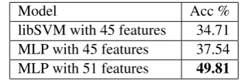
To evaluate the importance oflexicon-based fea-tures as well asemotion-weightfeatures, we use a simple multi-layer perceptron (MLP) model with 3 input, hidden andoutput layers. Two different models are trained by using two sets of features. While a tweet is represented using 45 lexicon-based features in the first model, they are rep-resented by adding emotion-weight features into our prior feature set in the second one. Thus, the inputs of the first and the second models are 45 and 51-dimensional vectors. We set the num-ber of hidden units as twice the input and assign them ReLU activation function. Finally, we ap-ply dropout with a rate of 0.5 to the output of the hidden layer and pass them to the output. The output layer consists of 6 units with sigmoid ac-tivation function. Table2shows the best accuracy

achieved from each of two models on the develop-ment set. From this table, we observe that adding 6 emotion-weight features to our lexicon-based fea-tures increases the accuracy from 37.54 to 49.81. Hence, we select the second model for the final system and also consider both feature sets in the other models. In order to make a comparison with linear models, we also used libSVM with linear kernel function in this experiment. As seen, MLP outperforms SVM when using 45 lexicon-based features.

Model Acc %

libSVM with 45 features 34.71 MLP with 45 features 37.54 MLP with 51 features 49.81

Table 2: The accuracy of SVM and MLP on the devel-opment set

2.4 Lexicon-Sensitive BiLSTM

In this section, we describe 2 types of deep neural network models using BiLSTM to predict the tar-get word emotion. First, we create a simple 4-layer neural network namelyinput,embedding,BiLSTM andoutput layers. Each tweet is represented se-quentially using 25K most frequent words. Those words out of vocabulary are treated as unknown word (UNK). However, the target word is not con-sidered as UNK. In all tweets, the target word is supposed as a single particular word that can ex-press all of the 6 emotions. In this model, pre-trained emotion-specific word vectors (described in Section 2.2) are used in the embedding layer. Here, a tweet which is represented as a sequence of word vectors is given to the BiLSTM layer in which the dimension of the hidden vectors in LSTM is 256. In order to avoid overfitting, we apply dropout (Srivastava et al.,2014) with a rate of 0.5 to the input of the BiLSTM layer. Finally, the output layer with 6 softmax units predicts the emotion of the target word.

Seq. Input (79)

Embedding Layer (79-200)

BLSTM Layer (512)

Output (Softmax Layer) (6)

Lexicon+emotion-weight

Input Features (51)

Concat. layer (563) with dropout 0.4

Figure 1: The architecture of Lexicon-BiLSTM ap-proach

neural network. Figure1depicts the overall archi-tecture of the proposed model. This approach is called as Lexicon-BiLSTM in our experiments.

2.5 Left-Right Context-Sensitive BiLSTM

In the three previous approaches, we actually clas-sified each tweet according to the emotion of the target word. However, in the fourth approach, we suppose the target word as a synthetic ambiguous word that can express 6 emotions depending on the context. Thus, our objective is to disambiguate the emotion expressed by this synthetic word in the given context (tweet). To this end, we consider the left and the right sides of the target word sep-arately. We extract two semantic vectors from the context of the target word by applying BiLSTM model to its left and right sides. Hence, we call this approach as Left-Right context-sensitive BiL-STM (LR-BiLBiL-STM). This exactly corresponds to the output of the BiLSTM layer in the two pre-vious models when only left or right context of the target word is considered as input. These two vectors together represent the semantic signature of the context in which target word has been oc-curred. By relying on these two vectors, we create a feed forward neural network to predict the emo-tion of the target word. In this network, the con-catenation of two semantic vectors are considered as input. The input is given to a hidden layer in which the number of units is the half of the input length. ReLU activation function is used in the hidden layer as well as two dropouts over its in-put and outin-put with rates of 0.5, 0.3 respectively. Finally, the output layer using 6 softmax units pre-dicts the emotion of the target word given its left and right contexts. Figure2 summarizes this ap-proach and shows the architecture of this model.

Left Seq.Input (61)

Shared Embedding Layer (79-200)

Left BLSTM (512)

Output (Softmax Layer) (6) Right Seq.Input (69)

Right BLSTM (512)

Hidden Layer (ReLU) (512) with dropout 0.3 Concat. layer (1024) with dropout 0.5

Figure 2: The architecture of LR-BiLSTM approach

2.6 Ensemble Approach-Final System

We proposed 4 different approaches in three pre-vious subsections. While 2 approaches leverage lexicon-based and emotion-weight features, two others only use hidden state vectors of the BiL-STM model. In order to use the advantages of all proposed models in the final system, we combine them using Bagging ensemble method (Breiman,

1996) to obtain an aggregated predictor. In this method, we take an average of the outputs of the proposed models and make a vote when predicting the emotion of the target word. Here, the output of each model is a6-dimensionalvector (one output per class). Thus,N models generate a matrixM

with the shape of N ×6. The output of the en-semble method is a6-dimensionalvector which is obtained by taking average of each column of ma-trixM. The class voting is done according to the maximum value of the result vector.

For the final system, we create 7 models based on 4 approaches proposed in Sections 2.3, 2.4

LR-BiLSTM-4). The architecture of LR-BiLSTM-4 is exactly the same as Figure 2. We use all these models in our final system since all of them in-creases the overall accuracy. For example, the system accuracy decreases to 67.4 without using Lexicon-MLP model.

3 Implementation Details

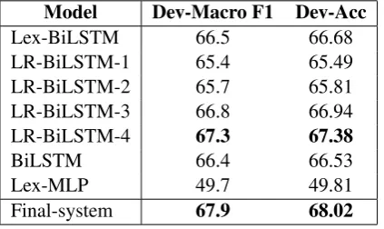
We used Keras library2 with TensorFlow back-end to implement all the proposed models. Be-fore training, we removed all urls, usernames and newlines inside a tweet and employed NLTK toolkit3 to tokenize tweets. All hyperparameters were tuned based on the development set with 50 epochs. We trained all models over training data provided by the shared task organizer (Klinger et al.,2018) and selected the best model based on the accuracy achieved from the development set. Table3shows the best results obtained by each of the proposed models.

Model Dev-Macro F1 Dev-Acc

Lex-BiLSTM 66.5 66.68

LR-BiLSTM-1 65.4 65.49

LR-BiLSTM-2 65.7 65.81

LR-BiLSTM-3 66.8 66.94

LR-BiLSTM-4 67.3 67.38

BiLSTM 66.4 66.53

Lex-MLP 49.7 49.81

Final-system 67.9 68.02

Table 3: The best results on the development set

4 Empirical Evaluation and Discussion

We evaluate the proposed models on the shared task official test set. Table4shows the results ac-cording to the shared task evaluation measures – micro and macro averaged F-measure– over all 6 emotion classes. According to the results, the pro-posed Left-Right context-sensitive BiLSTM ap-proach (i.e. LR-BiLSTM-3 and LR-BiLSTM-4) achieves the best official score of 67.8 among other individual models. The macro F1-score in-creases to 68.6 when using all models in our en-semble system.

According to the macro-F1 score achieved from BiLSTM and Lexicon-BiLSTM models, we can observe that two sets of lexicon-based and

2

https://keras.io/

3_{https://www.nltk.org/}

emotion-weight features improve the performance of BiLSTM model. However, this growth is not seen in all classes. For example, in two joy andsad classes, BiLSTM model performs better than Lexicon-BiLSTM. In addition, the macro and micro averaged F-measure values obtained from the Lexicon-MLP (see Table 4) indicate that the lexicon-based and emotion-weight features are ef-fective on less than 50% of test instances. This can raise two facts about the test set (1) a small number of affective clue words are used in the tweets (2) the syntactic structure of the context changes the emotions expressed by the affective clue words in the tweets. This issue will be further discussed in Section4.1.

Another important finding is that all models give a weak performance on the anger and sur-prise emotions. The confusion matrix shown in Table 5 indicates that our final system predicts tweets as anger instead of surprisein 402 cases and vice versa in 519 cases. These are the highest False Negative (FN) errors with respect toanger andsurpriseemotion classes and show that these two emotions occur in similar contexts. It means that the senses expressed by these two emotion classes are much similar to each other in some tweets in which our system cannot distinguish them from each other. Moreover, from Table 5, anger andsurpriseemotions constitute the high-est portion of the FN errors in the other emotion classes. They are bold in Table5.

4.1 Error Analysis

We analyze the errors of the final system from two different aspects. In the first one, none of the mod-els predict the correct emotion, whereas in the sec-ond one at least one model predict correctly. Here, we give two examples for each case, respectively:

• Ex.1 “I don’t understand why everyone’s [#TRIGGERWORD#] when Miley shows her body she’s comfortable so why should it matter to you?”

• Ex.2 “it is quite [#TRIGGERWORD#] that you think that is awesome.”

• Ex.3 “Cold coffee is really only [#TRIG-GERWORD#] when you expect it to be hot. Otherwise, it’s just as good.”

• Ex.4 “@USERNAME making me

Models F1-score over emotion classes Mic-avg Mac-avg

surp. disg. sad fear anger joy (official)

Lex-BiLSTM 63.7 67.5 64.9 70.3 60.5 76.2 67.4 67.2

LR-BiLSTM-1 61.8 65.5 63.6 68.2 58.6 75.1 65.6 65.5

LR-BiLSTM-2 61.7 66.3 62.8 68.9 59.1 74.9 65.8 65.6

LR-BiLSTM-3 63.8 68.1 66.3 71.0 60.2 77.3 68.0 67.8

LR-BiLSTM-4 64.2 68.3 65.6 70.8 60.9 76.9 67.9 67.8

BiLSTM 63.6 67.0 65.2 69.5 59.5 76.3 67.0 66.9

Lex-MLP 42.7 53.5 45.4 50.8 43.2 61.1 49.6 49.4

Final-system 64.9 69.0 66.4 71.6 62.3 77.6 68.8 68.6

Table 4: The performance of all models on the official test set

Predict

Real surp. disg. sad fear anger joy

surp. 3310 367 183 303 402 227

disg. 554 3246 312 158 380 144

sad 236 384 2762 207 430 321

fear 494 177 192 3337 368 223

anger 519 336 297 326 3033 283

joy 289 103 228 203 336 4087

Table 5: Confusion matrix for final system

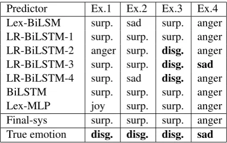
Table 6 indicates the predictions of the pro-posed models for the four above examples along with their true emotion labels. From the confu-sion matrix (Table 5) the biggest number of er-rors occurs when our system predict a tweet as surprise, whereas the true emotion isdisgust(554 cases). Hence, the three of above examples were selected from the disgust class and last one was selected from sad. In Ex.1, it is observed that most of the models predict the emotion of the tar-get word assurprise. However, Lexicon-MLP and LR-BiLSTM-2 predict it asjoyandanger, respec-tively. Since Lexicon-MLP only use the lexicon-based and emotion-weight features, it cannot pre-dict correctly when the emotion of the target word depends on the syntactic and semantic structures of the tweet. Thus, it predicts an opposite emotion (i.e. joy) for Ex.1. Moreover, you can see an am-biguity amongsurprise,angeranddisgustin this example. In Ex.2, there is an irony that makes dif-ficult the recognition of the target word emotion. Although the Ex.3 is similar to Ex.1, our context-sensitive BiLSTM approach (LR-BiLSTM-4) pre-dicts the correct emotion. In Ex.4, you can see a challenge between anger and sad emotions. All the proposed models predict the emotion of the target word as anger except for LR-BiLSTM-3

which correctly predicts the target word emotion assad. Here, we believe that a mixed emotion is inferred from the given context in Ex.4. However, the length of tweets is limited, thus it makes diffi-cult the disambiguation task for the implicit emo-tion recogniemo-tion.

Predictor Ex.1 Ex.2 Ex.3 Ex.4

Lex-BiLSM surp. sad surp. anger

LR-BiLSTM-1 surp. surp. surp. anger

LR-BiLSTM-2 anger surp. disg. anger

LR-BiLSTM-3 surp. surp. disg. sad

LR-BiLSTM-4 surp. sad disg. anger

BiLSTM surp. surp. surp. anger

Lex-MLP joy surp. surp. anger

Final-sys surp. surp. surp. anger

True emotion disg. disg. disg. sad

Table 6: The predictions of models on 4 samples of tweets in the test set

5 Conclusion

References

Muhammad Abdul-Mageed and Lyle Ungar. 2017. Emonet: Fine-grained emotion detection with gated recurrent neural networks. In Proceedings of the 55th Annual Meeting of the Association for Compu-tational Linguistics (Volume 1: Long Papers), vol-ume 1, pages 718–728.

Leo Breiman. 1996. Bagging predictors. Machine learning, 24(2):123–140.

Paul Ekman. 1992. An argument for basic emotions.

Cognition & emotion, 6(3-4):169–200.

Nal Kalchbrenner, Edward Grefenstette, and Phil Blunsom. 2014. A convolutional neural net-work for modelling sentences. arXiv preprint arXiv:1404.2188.

Sunghwan Mac Kim, Alessandro Valitutti, and Rafael A Calvo. 2010. Evaluation of unsupervised emotion models to textual affect recognition. In

Proceedings of the NAACL HLT 2010 Workshop on Computational Approaches to Analysis and Gener-ation of Emotion in Text, pages 62–70. Association for Computational Linguistics.

Roman Klinger, Orph´ee de Clercq, Saif M. Moham-mad, and Alexandra Balahur. 2018. IEST: WASSA-2018 Implicit Emotions Shared Task. In Proceed-ings of the 9th Workshop on Computational Ap-proaches to Subjectivity, Sentiment and Social Me-dia Analysis, Brussels, Belgium. Association for Computational Linguistics.

Maximilian K¨oper, Evgeny Kim, and Roman Klinger. 2017. IMS at EmoInt-2017: emotion intensity pre-diction with affective norms, automatically extended resources and deep learning. In Proceedings of the 8th Workshop on Computational Approaches to Subjectivity, Sentiment and Social Media Analysis, pages 50–57.

Sophia Yat Mei Lee, Ying Chen, and Chu-Ren Huang. 2010. A text-driven rule-based system for emotion cause detection. InProceedings of the NAACL HLT 2010 Workshop on Computational Approaches to Analysis and Generation of Emotion in Text, pages 45–53. Association for Computational Linguistics.

Jasy Suet Yan Liew and Howard R Turtle. 2016. Ex-ploring fine-grained emotion detection in tweets. In

Proceedings of the NAACL Student Research Work-shop, pages 73–80.

Saif M Mohammad and Felipe Bravo-Marquez. 2017. WASSA-2017 shared task on emotion intensity.

arXiv preprint arXiv:1708.03700.

Saif M Mohammad, Svetlana Kiritchenko, and Xiao-dan Zhu. 2013. NRC-Canada: Building the state-of-the-art in sentiment analysis of tweets. arXiv preprint arXiv:1308.6242.

Behzad Naderalvojoud, Ebru Akcapinar Sezer, and Alaettin Ucan. 2015. Imbalanced text categoriza-tion based on positive and negative term weight-ing approach. InInternational Conference on Text, Speech, and Dialogue, pages 325–333. Springer.

Nitish Srivastava, Geoffrey Hinton, Alex Krizhevsky, Ilya Sutskever, and Ruslan Salakhutdinov. 2014. Dropout: a simple way to prevent neural networks from overfitting. The Journal of Machine Learning Research, 15(1):1929–1958.

Dario Stojanovski, Gjorgji Strezoski, Gjorgji Mad-jarov, and Ivica Dimitrovski. 2016. Finki at semeval-2016 task 4: Deep learning architecture for twitter sentiment analysis. In Proceedings of the 10th International workshop on semantic evaluation (SemEval-2016), pages 149–154.

Carlo Strapparava, Alessandro Valitutti, et al. 2004. Wordnet affect: an affective extension of wordnet. InLrec, volume 4, pages 1083–1086. Citeseer.

Duyu Tang, Furu Wei, Nan Yang, Ming Zhou, Ting Liu, and Bing Qin. 2014. Learning sentiment-specific word embedding for twitter sentiment clas-sification. InProceedings of the 52nd Annual Meet-ing of the Association for Computational LMeet-inguistics (Volume 1: Long Papers), volume 1, pages 1555– 1565.

Jin Wang, Liang-Chih Yu, K Robert Lai, and Xue-jie Zhang. 2016. Dimensional sentiment analysis using a regional CNN-LSTM model. In Proceed-ings of the 54th Annual Meeting of the Association for Computational Linguistics (Volume 2: Short Pa-pers), volume 2, pages 225–230.