Ngram2vec: Learning Improved Word Representations from Ngram Co occurrence Statistics

Ngram2vec: Learning Improved Word Representations from Ngram

Co-occurrence Statistics

Zhe Zhao1,2

[email protected] Tao Liu

1,2 [email protected]

Shen Li3,4

[email protected] Bofang Li

1,2

[email protected] Xiaoyong Du

1,2 [email protected]

1_{School of Information, Renmin University of China}

2_{Key Laboratory of Data Engineering and Knowledge Engineering, MOE} 3_{Institute of Chinese Information Processing, Beijing Normal University}

4_{UltraPower-BNU Joint Laboratory for Artificial Intelligence, Beijing Normal University}

Abstract

The existing word representation method-s momethod-stly limit their information method-source to word co-occurrence statistics. In this pa-per, we introduce ngrams into four repre-sentation methods: SGNS, GloVe, PPMI matrix, and its SVD factorization. Com-prehensive experiments are conducted on word analogy and similarity tasks. The results show that improved word repre-sentations are learned from ngram co-occurrence statistics. We also demonstrate that the trained ngram representations are useful in many aspects such as finding antonyms and collocations. Besides, a novel approach of building co-occurrence matrix is proposed to alleviate the hard-ware burdens brought by ngrams.

1 Introduction

Recently, deep learning approaches have achieved state-of-the-art results on a range of NLP tasks. One of the most fundamental work in this field is word embedding, where low-dimensional word representations are learned from unlabeled corpo-ra through neucorpo-ral models. The tcorpo-rained word em-beddings reflect semantic and syntactic informa-tion of words. They are not only useful in reveal-ing lexical semantics, but also used as inputs of various downstream tasks for better performance (Kim, 2014; Collobert et al., 2011; Pennington et al.,2014).

Most of the word embedding models are trained upon <word, context> pairs in the local win-dow. Among them, word2vec gains its popu-larity by its amazing effectiveness and efficien-cy (Mikolov et al., 2013b,a). It achieves

state-of-the-art results on a range of linguistic tasks with only a fraction of time compared with pre-vious techniques. A challenger of word2vec is GloVe (Pennington et al.,2014). Instead of train-ing on<word, context>pairs, GloVe directly uti-lizes word co-occurrence matrix. They claim that the change brings the improvement over word2vec on both accuracy and speed. Levy and Goldberg

(2014b) further reveal that the attractive properties observed in word embeddings are not restricted to neural models such as word2vec and GloVe. They use traditional count-based method (PPMI matrix with hyper-parameter tuning) to represent word-s, and achieve comparable results with the above neural embedding models.

The above models limit their information source to word co-occurrence statistics (Levy et al.,

2015). To learn improved word representation-s, we extend the information source from co-occurrence of‘word-word’ type to co-occurrence of‘ngram-ngram’type. The idea of using ngrams is well supported by language modeling, one of the oldest problems studied in statistical NLP. In lan-guage models, co-occurrence of words and ngrams is used to predict the next word (Kneser and Ney,

1995;Katz,1987). Actually, the idea of word em-bedding models roots in language models. They are closely related but are used for different pur-poses. Word embedding models aim at learning useful word representations instead of word pre-diction. Since ngram is a vital part in language modeling, we are inspired to integrate ngram sta-tistical information into the recent word represen-tation methods for better performance.

The idea of using ngrams is intuitive. However, there is still rare work using ngrams in recent rep-resentation methods. In this paper, we introduce

ngrams into SGNS, GloVe, PPMI, and its SVD factorization. To evaluate the ngram-based mod-els, comprehensive experiments are conducted on word analogy and similarity tasks. Experimental results demonstrate that the improved word repre-sentations are learned from ngram co-occurrence statistics. Besides that, we qualitatively evaluate the trained ngram representations. We show that they are able to reflect ngrams’ meanings and syn-tactic patterns (e.g. ‘be + past participle’ pattern). The high-quality ngram representations are useful in many ways. For example, ngrams in negative form (e.g. ‘not interesting’) can be used for find-ing antonyms (e.g. ‘borfind-ing’).

Finally, a novel method is proposed to build n-gram co-occurrence matrix. Our method reduces the disk I/O as much as possible, largely alle-viating the costs brought by ngrams. We uni-fy different representation methods in a pipeline. The source code is organized asngram2vec toolk-it and released at https://github.com/ zhezhaoa/ngram2vec.

2 Related Work

SGNS, GloVe, PPMI, and its SVD factorization are used as baselines. The information used by them does not go beyond word co-occurrence s-tatistics. However, their approaches to using the information are different. We review these meth-ods in the following 3 sections. In section 2.4, we revisit the use of ngrams in the deep learning con-text.

2.1 SGNS

Skip-gram with negative sampling (SGNS) is a model in word2vec toolkit (Mikolov et al.,

2013b,a). Its training procedure follows the ma-jority of neural embedding models (Bengio et al.,

2003): (1) Scan the corpus and use <word, context> pairs in the local window as training samples. (2)Train the models to make words use-ful for predicting contexts (or in reverse). The de-tails of SGNS is discussed in Section 3.1. Com-pared to previous neural embedding models, S-GNS speeds up the training process, reducing the training time from days or weeks to hours. Also, the trained embeddings possess attractive proper-ties. They are able to reflect relations between two words accurately, which is evaluated by a fancy task called word analogy.

Due to the above advantages, many models are

proposed on the basis of SGNS. For example,

Faruqui et al.(2015) introduce knowledge in lex-ical resources into the models in word2vec. Zhao et al. (2016) extend the contexts from the local window to the entire documents. Li et al.(2015) use supervised information to guide the training. Dependency parse-tree is used for defining contex-t in (Levy and Goldberg, 2014a). LSTM is used for modeling context in (Melamud et al., 2016) Sub-word information is considered in (Sun et al.,

2016;Soricut and Och,2015).

2.2 GloVe

Different from typical neural embedding model-s which are trained on <word, context> pairs, GloVe learns word representation on the basis of co-occurrence matrix (Pennington et al., 2014). GloVe breaks traditional ‘words predict contexts’ paradigm. Its objective is to reconstruct non-zero values in the matrix. The direct use of matrix is reported to bring improved results and higher speed. However, there is still dispute about the advantages of GloVe over word2vec (Levy et al.,

2015;Schnabel et al.,2015). GloVe and other em-bedding models are essentially based on word co-occurrence statistics of the corpus. The <word, context> pairs and co-occurrence matrix can be converted to each other.Suzuki and Nagata(2015) try to unify GloVe and SGNS in one framework.

2.3 PPMI & SVD

When we are satisfied with the huge promotions achieved by embedding models on linguistic tasks, a natural question is raised: where the superior-ities come from. One conjecture is that it’s due to the neural networks. However,Levy and Gold-berg(2014c) reveal that SGNS is just factoring P-MI matrix implicitly. Also, Levy and Goldberg

(2014b) show that positive PMI (PPMI) matrix still rivals the newly proposed embedding mod-els on a range of linguistic tasks. Properties like word analogy are not restricted to neural model-s. To obtain dense word representations from PP-MI matrix, we factorize PPPP-MI matrix with SVD, a classic dimensionality reduction method for learn-ing low-dimensional vectors from sparse matrix (Deerwester et al.,1990).

2.4 Ngram in Deep Learning

reported to perform well on a range of NLP tasks (Blunsom et al.,2014;Hu et al.,2014;Severyn and Moschitti, 2015). CNNs are essentially using n-gram information to represent texts. They use 1-D convolutional layers to extract ngram features and the distinct features are selected by max-pooling layers. In (Li et al.,2016), ngram embedding is in-troduced into Paragraph Vector model, where tex-t embedding is tex-trained tex-to be useful tex-to predictex-t n-grams in the text. In the word embedding liter-ature, a related work is done by Melamud et al.

(2014), where word embedding models are used as baselines. They propose to use ngram language models to model the context, showing the effec-tiveness of ngrams on similarity tasks. Another work that is related to ngram is fromMikolov et al.

(2013b), where phrases are embedded into vec-tors. It should be noted that phrases are different from ngrams. Phrases have clear semantics and the number of phrases is much less than the num-ber of ngrams. Using phrase embedding has little impact on word embedding’s quality.

3 Model

In this section, we introduce ngrams into SGNS, GloVe, PPMI, and SVD. Section 3.1 reviews the SGNS. Section 3.2 and 3.3 show the details of in-troducing ngrams into SGNS. In section 3.4, we show the way of using ngrams in GloVe, PPMI, and SVD, and propose a novel way of building n-gram co-occurrence matrix.

3.1 Word Predicts Word: the Revisit of SGNS

First we establish some notations. The raw input is a corpus T ={w1,w2,...,w|T|}. Let W andC denote word and context vocabularies.θis the pa-rameters to be optimized. SGNS’s papa-rameters in-volve two parts: word embedding matrix and con-text embedding matrix. With embedding ~w∈Rd_,

the total number of parameters is(|W|+|C|)*d. The SGNS’s objective is to maximize the condi-tional probabilities of contexts given center words:

|T|

X

t=1

" X

c∈C(wt)

log p(c|wt;θ)

#

(1)

where C(wt) ={wi, t−win≤i≤t+win and i6=t}

and win denotes the window size. As illustrat-ed in figure 1, the center word ‘written’ prillustrat-edict- predict-s itpredict-s predict-surrounding wordpredict-s ‘Potter’, ‘ipredict-s’, ‘by’, and

Figure 1: Illustration of ‘word predicts word’.

‘J.K.’. In this paper, negative sampling (Mikolov et al.,2013b) is used to approximate the condition-al probability:

p(c|w) =σ(~wT_~c)Yk j=1

E_cj∼Pn(C)σ(−~wT_~c j) (2)

whereσ is sigmoid function. k samples (fromc1 tock) are drawn from context distribution raised

to the power ofn.

3.2 Word Predicts Ngram

In this section, we introduce ngrams into context vocabulary. We treat each ngram as a normal word and give it a unique embedding. During the train-ing, the center word should not only predict its sur-rounding words, but also predict its sursur-rounding n-grams. As shown in figure 2, center word ‘written’ predicts the bigrams in the local window such as ‘by J.K.’. The objective of ‘word predicts ngram’ is similar with the original SGNS. The only differ-ence is the definition of theC(w). In ngram case, C(w)is formally defined as follows:

C(wt) = N S

n=1{wi:i+n|wi:i+nis not wtAND

t−win≤i≤t+win−n+ 1} (3)

Figure 2: Illustration of ‘word predicts ngram’.

ngram ‘is written’ and ‘written by’ are predicted by the center word ‘written’. In the non-overlap case, these ngrams are excluded. The properties of word embeddings are different when overlap is allowed or not, which will be discussed in experi-ments section.

3.3 Ngram Predicts Ngram

We further extend the model to introduce ngram-s into center word vocabulary. During the train-ing, center ngrams (including words) predict their surrounding ngrams. As shown in figure 3, center bigram ‘is written’ predicts its surrounding word-s and bigramword-s. The objective of ‘ngram predictword-s ngram’ is as follows:

|T|

X

t=1

Nw X

nw=1 "

X

c∈C(wt:t+nw)

log p(c|wt:t+nw;θ) #

(4)

whereNw is the order of center ngram. The

defi-nition ofC(wt:t+nw)is as follows:

Nc

S

nc=1{wi:i+nc|wi:i+nc is not wt:t+nw AND

t−win+nw−1≤i≤t+win−nc+ 1}

(5)

where Nc is the order of context ngram. To this

end, the word embeddings are not only affected by the ngrams in the context, but also indirect-ly affected by co-occurrence statistics of ‘ngram-ngram’ type in the corpus.

SGNS is proven to be equivalent with factor-izing pointwise mutual information (PMI) ma-trix (Levy and Goldberg,2014c). Following their work, we can easily show that models in section 3.2 and 3.3 are implicitly factoring PMI matrix of ‘word-ngram’ and ‘ngram-ngram’ type. In the next section, we will discuss the content of intro-ducing ngrams into positive PMI (PPMI) matrix.

3.4 Co-occurrence Matrix Construction

Introducing ngrams into GloVe, PPMI, and SVD is straightforward: the only change is to replace

Figure 3: Illustration of ‘ngram predicts ngram’.

word co-occurrence matrices with ngram ones. In the above three sections, we have discussed the way of taking out<word(ngram), word(ngram)> pairs from a corpus. Afterwards, we build the co-occurrence matrix upon these pairs. The rest steps are identical with the original baseline models.

Win Type #Pairs

2 uni uniuni bi 0.36B1.14B

uni tri 1.40B

bi bi 2.78B

bi tri 3.65B

5 uni uniuni bi 0.91B2.79B

uni tri 3.81B

bi bi 7.97B

Table 1: The number of pairs at different settings. The type column lists the order of ngrams consid-ered in center word/context vocabularies. For ex-ample, uni bi denotes that center word vocabulary contains unigrams (words) and context vocabulary contains both unigrams and bigrams. The setting of other hyper-parameters is discussed in Section 4.2.

However, building the co-occurrence matrix is not an easy task as it apparently looks like. The introduction of ngrams brings huge burdens on the hardware. The matrix construction cost is closely related to the number of pairs (#Pairs). Table 1 shows the statistics of pairs extracted from corpus wiki20101_{. We can observe that#Pairs is huge} when ngrams are considered.

To speed up the process of building ngram co-occurrence matrix, we take advantages of ‘mixture’ strategy (Pennington et al., 2014) and ‘stripes’ strategy (Dyer et al., 2008; Lin, 2008). The two strategies optimize the process in differ-ent aspects. Computational cost is reduced signif-icantly when they are used together.

When words (or ngrams) are sorted in descend-ing order by frequency, the co-occurrence matrix’s top-left corner is dense while the rest part is s-parse. Based on this observation, the ‘mixture’ of two data structures are used for storing ma-trix. Elements in the top-left corner are stored in a 2D array, which stays in memory. The rest of the elements are stored in the form of <ngram, H>, where H<context, count> is an associative array recording the number of times thengramand context co-occurs (‘stripes’ strategy). Compared with storing <ngram, context> pairs explicitly, the ‘stripes’ strategy provides more opportunities to aggregate pairs outside of the top-left corner.

Algorithm 1 shows the way of using the ‘mix-ture’ and ‘stripes’ strategies together. In the first stage, pairs are stored in different data structures according totopLeftfunction. Intermediate results are written to temporary files when memory is full. In the second stage, we merge these sorted tempo-rary files to generate co-occurrence matrix. The getSmallest function takes out the pair <ngram, H>with the smallestkeyfrom temporary files. In practice, algorithm 1 is efficient. Instead of using computer clusters (Lin, 2008), we can build the matrix of ‘bi bi’ type even in a laptop. It only re-quires 12GB to store temporary files (win=2, sub-sampling=0, memory size=4GB), which is much smaller than the implementations in (Pennington et al., 2014; Levy et al., 2015) . More detailed analysis about these strategies can be found in the

ngram2vectoolkit.

4 Experiments

4.1 Datasets

The tasks used in this paper is the same with the work ofLevy et al.(2015), including six similarity and two analogy datasets. In similarity task, a s-calar (e.g. a score from 0 to 10) is used to measure the relation between the two words. For example, in a similarity dataset, the ‘train, car’ pair is giv-en the score of 6.31. A problem of similarity task is that scalar only reflects the strength of the rela-tion, while the type of relation is totally ignored (Schnabel et al.,2015).

Due to the deficiency of similarity task, anal-ogy task is widely used as benchmark recently for evaluation of word embedding models. To answer analogy questions, relations between the two words are reflected by a vector, which is usually obtained by the difference between word

Algorithm 1: An algorithm for building n-gram co-occurrence matrix

Input : PairsP, Sorted vocabularyV

Output: Sorted and aggregated pairs

1 The 2D arrayA[ ][ ];

2 The dictionaryD < ngram, H >; 3 The temporary files arraytfs[ ];fid=1; 4 forpairp < n, c >inPdo

5 iftopLeft(n, c) == 1then 6 A[getId(n)][getId(c)]+= 1; 7 else

8 D{n}{c}+= 1;

9 ifMemory is fullorP is emptythen 10 SortDby key (ngram); 11 WriteDtotfs[fid];

12 fid+= 1;

13 end

14 end

15 end

16 WriteAtotfs[0]in the form of< ngram, H >; 17 old=getSmallest(tfs) ;

18 while!(All files intfsare empty)do 19 new=getSmallest(tfs) ; 20 ifold.ngram==new.ngramthen

21 old=

< old.ngram, merge(old.H, new.H)>;

22 else

23 Writeoldto disk;

24 old=new

25 end

26 end

embeddings. Different from a scalar, the vec-tor provides more accurate descriptions of rela-tions. For example, capital-country relation is encoded in vec(Athens)-vec(Greece), vec(Tokyo)-vec(Japan)and so on. More concretely, the ques-tions in the analogy task are in the form of ‘a is to b as c is to d’. ‘d’ is an unknown word in the test phase. To correctly answer the questions, the models should embed the two relations, vec(a)-vec(b)andvec(c)-vec(d), into similar positions in the space. Following the work ofLevy and Gold-berg(2014b), both additive (add) and multiplica-tive (mul) functions are used for finding word ‘d’. The latter one is more suitable for sparse represen-tation in practice.

4.2 Pipeline and Hyper-parameter Setting

Win Type Google Tot. / Sem. / Syn._{Add Mul Add}MSR_Mul

2

uni uni .579 / .543 / .608 .597 / .561 / .627 .513 .533 overlap _{uni tri}uni bi .587 / .651 / .533_{.505 / .615 / .414} .626 / .681 / .580_{.553 / .657 / .466} .473_.358 .508_.396 bi bi .664/.739/ .602 .680/.739/ .631 .547 .575 bi tri .572 / .695 / .470 .601 / .713 / .508 .416 .447 non-overlap uni bi_{bi bi} .610 / .558 / .653_{.644 / .607 /.674} .633 / .581 / .676_{.659 / .613 /.696} .568_.590 .595_.616

5

uni uni .653 / .669 / .639 .668 / .678 / .660 .511 .535 overlap _{uni tri}uni bi .696 / .745 / .655_{.679 / .738 / .630} .714 / .752 / .683_{.699 / .750 / .657} .518_.542 .542_.549 bi bi .704 /.764/ .654 .718 /.764/ .681 .537 .560 non-overlap _{uni tri}uni bi .696 / .722 / .675_{.687 / .711 / .668} .716 / .731 / .703_{.705 / .717 / .696} .549_.542 .579_.574 bi bi .712/ .745 /.684 .725/ .742 /.710 .569 .607

Table 2: Performance of (ngram) SGNS on analogy datasets.

Win Type Sim. Rel. Bruni Radinsky Luong Hill 2 uni uniuni bi .745.739 .586.600 .713.698 .635.627 .387.395 .419.429

uni tri .700 .535 .658 .591 .380 .415 bi bi .757 .574 .724 .644 .408 .407 bi tri .724 .564 .669 .605 .403 .412 5 uni uniuni bi .789.794 .648.681 .756.752 .652.653 .407.437 .401.431 uni tri .783 .673 .743 .652 .432 .436

bi bi .816 .703 .760 .671 .446 .421 Table 3: Performance of (ngram) SGNS on similarity datasets.

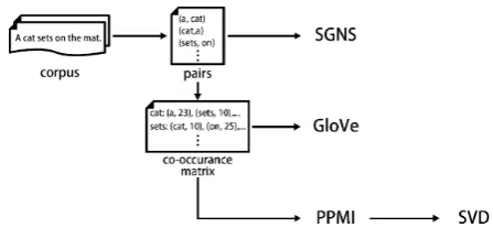
Figure 4: The pipeline.

matrix. SVD factorizes the PPMI matrix to obtain low-dimensional representation.

Most hyper-parameters come from ‘corpus to pairs’ part and four representation models. ‘corpus to pairs’ part determines the source of information for the subsequent models and its hyper-parameter setting is as follows: low-frequency words (n-grams) are removed with a threshold of 10. High-frequency words (ngrams) are removed with sub-sampling at the degree of 1e-5 2_{. Window size} is set to 2 and 5. Clean strategy (Levy et al.,

2015) is used to ensure no information beyond

2_{Sub-sampling is not used in GloVe, which follows its} o-riginal setting.

pre-specified window is included. Overlap setting is used in default. For hyper-parameters of four representation models, we use the embeddings of 300 dimensions in dense representations. SGNS is trained by 3 iterations. The rest strictly follow the baseline models3_{. We consider unigrams (words),} bigrams, and trigrams in this work. The imple-mentation of higher-order models and their results will be released withngram2vectoolkit.

4.3 Ngrams on SGNS

SGNS is a popular word embedding model. Even compared with its challengers such as GloVe, S-GNS is reported to have more robust performance with faster training speed (Levy et al.,2015). Ta-ble 2 lists the results on analogy datasets. We can observe that the introduction of bigrams pro-vides significant improvements at different hyper-parameter settings. The SGNS of ‘bi bi’ type pro-vides the highest results. It is very effective on capturing semantic information (Google seman-tic). Around 10 percent improvements are

wit-3_{http://bitbucket.org/omerlevy/}

hyperwordsfor SGNS, PPMI and SVD;

http://nlp.stanford.edu/projects/glove/

Win Type _Add Google _{Mul Add}MSR_Mul Sim. Rel. Bruni Radinsky Luong Hill

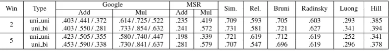
2 uni uni_{uni bi} .403 / .441 / .372_{.403 / .550 / .281} .614 / .725 / .522_{.733 / .854 / .632} .235_{.241 .572}.419 _.731.709 _.581.593 _.721.705 _.627.603 _.341.293 .385_.394

5 uni uni_{uni bi} .423 / .505 / .355_{.453 / .590 / .338} .580 / .740 / .447_{.730 / .841 / .637} .198_{.281 .579}.339 _.707.721 _.547.619 _.696.712 _.619.619 _.296.252 .341_.378

Table 4: Performance of (ngram) PPMI on analogy and similarity datasets.

Win Type _Add Google _{Mul Add}MSR_Mul Sim. Rel. Bruni Radinsky Luong Hill

2 uni uni_{uni bi} .535 / .599 / .482_{.543 / .601 / .493} .540 / .610 / .481_{.549 / .612 / .496} .444_{.464 .472}.445 _.686.681 _.545.529 _.695.698 _.631.608 _.389.381 .351_.352

5 uni uni_{uni bi} .625 / .689 / .572_{.631 / .699 / .575} .626 / .696 / .568_{.633 / .703 / .574} .476_{.477 .504}.490 _.752.747 _.610.600 _.737.735 _.631.657 _.395.389 .347_.342

Table 5: Performance of (ngram) GloVe on analogy and similarity datasets.

Win Type _Add Google _{Mul Add}MSR_Mul Sim. Rel. Bruni Radinsky Luong Hill

2 uni uni_{uni bi} .419 / .388 / .446_{.387 / .322 / .440} .439 / .394 / .477_{.410 / .327 / .479} .321_{.372 .402}.353 _.739.714 _.546.593 _.688.712 _.636.625 _.427.410 .344_.347

5 uni uni_{uni bi} .433 / .426 / .439_{.410 / .340 / .468} .460 / .463 / .458_{.446 / .365 / .513} .290_{.374 .416}.321 _.751.752 _.559.633 _.698.731 _.639.623 _.426.411 .326_.363

Table 6: Performance of (ngram) SVD on analogy and similarity datasets.

nessed on semantic questions compared with u-ni uu-ni baseline. For syntactic questions (Google syntactic and MSR datasets), around 5 percent im-provements are obtained on average.

The effect of overlap is large on analogy datasets. Semantic questions prefer the overlap setting. Around 10 and 3 percent improvements are witnessed compared with non-overlap setting at the window size of 2 and 5. While in syntac-tic case, non-overlap setting performs better by a margin of around 5 percent.

The introduction of trigrams deteriorates the models’ performance on analogy datasets (espe-cially at the window size of 2). It is probably be-cause that trigram is sparse on wiki2010, a rela-tively small corpus with 1 billion tokens. We con-jecture that high order ngrams are more suitable for large corpora and will report the results in our future work. It should be noticed that trigram is not included in vocabulary in non-overlap case at the window size of 2. The shortest distance be-tween a word and a trigram is 3, which exceeds the window size.

Table 3 illustrates the SGNS’s performance on similarity task. The conclusion is similar with the case in analogy datasets. The use of bigrams is effective while the introduction of trigrams deteri-orates the performance in most cases. In general, the bigrams bring significant improvements over SGNS on a range of linguistic tasks. It is gener-ally known that ngram is a vital part in tradition-al language modeling problem. Results in table 2

and 3 confirm the effectiveness of ngrams again on SGNS, a more advanced word embedding model.

4.4 Ngrams on PPMI, GloVe, SVD

In this section, we only report the results of mod-els of ‘uni uni’ and ‘uni bi’ types. Using high-er ordhigh-er co-occurrence statistics brings immense costs (especially at the window size of 5). Levy and Goldberg(2014b) demonstrate that traditional count-based models can still achieve competitive results on many linguistic tasks, challenging the dominance of neural embedding models. Table 4 lists the results of PPMI matrix on analogy and similarity datasets. PPMI prefers Multiplicative (Mul) evalution. To this end, we focus on analyz-ing the results on Mul columns. When bigrams are used, significant improvements are witnessed on analogy task. On Google dataset, bigrams bring over 10 percent increase on the total accuracies. At the window size of 2, the accuracy in semantic questions even reaches 0.854, which is the state-of-the-art result to the best of our knowledge. On MSR dataset, around 20 percent improvements are achieved. The use of bigrams does not always bring improvements on similarity datasets. PPMI matrix of ‘uni bi’ type improves the results on 5 datasets at the window size of 2. At the window size of 5, using bigrams only improves the results on 2 datasets.

of bigrams. On similarity datasets, improvements are witnessed on most cases. For SVD, bigram-s bigram-sometimebigram-s lead to worbigram-se rebigram-sultbigram-s in both anal-ogy and similarity tasks. In general, significan-t improvemensignifican-ts are nosignifican-t wisignifican-tnessed on GloVe and SVD. Our preliminary conjecture is that the de-fault hyper-parameter setting should be blamed. We strictly follow the hyper-parameters used in baseline models, making no adjustments to cater to the introduction of ngrams. Besides that, some common techniques such as dynamic window, de-creasing weighting function, dirty sub-sampling are discarded. The relationships between ngrams and various hyper-parameters require further ex-ploration. Though trivial, it may lead to much bet-ter results and give researchers betbet-ter understand-ing of different representation methods. That will be the focus of our future work.

4.5 Qualitative Evaluations of Ngram Embedding

In this section, we analyze the properties of n-gram embeddings trained by SGNS of ‘bi bi’ type. Ideally, the trained ngram embeddings should re-flect ngrams’ semantic meanings. For example, vec(wasn’t able) should be close to vec(unable). vec(is written) should be close to vec(write) and vec(book). Also, the trained ngram embeddings should preserve ngrams’ syntactic patterns. For example, ‘was written’ is in the form of ‘be + past participle’ and the nearest neighbors should pos-sess similar patterns, such as ‘is written’ and ‘was transcribed’.

Table 7 lists the target ngrams and their top n-earest neighbours. We divide the target ngram-s into ngram-six groupngram-s according to their patternngram-s. We can observe that the returned words and ngram-s are very intuitive. Angram-s might be expected, ngram- syn-onyms of the target ngrams are returned in top po-sitions (e.g. ‘give off’ and ‘emit’; ‘heavy rain’ and ‘downpours’). From the results of the first group, it can be observed that bigram in negative form ‘not X’ is useful for finding the antonym of word ‘X’. Besides that, the trained ngram embeddings also preserve some common sense. For example, the returned result of ‘highest mountain’ is a list of mountain names (with a few exceptions such as ‘unclimbed’). In terms of syntactic patterns, we can observe that in most cases, the returned ngrams are in the similar form with target ngram-s. In general, the trained embeddings basically

re-flect semantic meanings and syntactic patterns of ngrams.

With high-quality ngram embeddings, we have the opportunity to do more interesting things in our future work. For example, we will construct a antonym dataset to evaluate ngram embeddings systematically. Besides that, we will find more scenarios for using ngram embeddings. In our view, ngram embeddings have potential to be used in many NLP tasks. For example, Johnson and Zhang(2015) use one-hot ngram representation as the input of CNN.Li et al.(2016) use ngram em-beddings to represent texts. Intuitively, initializing these models with pre-trained ngram embeddings may further improve the accuracies.

5 Conclusion

We introduce ngrams into four representation methods. The experimental results demonstrate n-grams’ effectiveness for learning improved word representations. In addition, we find that the trained ngram embeddings are able to reflect their semantic meanings and syntactic patterns. To al-leviate the costs brought by ngrams, we propose a novel way of building co-occurrence matrix, en-abling the ngram-based models to run on cheap hardware.

Acknowledgments

This work is supported by National Natural Sci-ence Foundation of China (Grant No. 61472428 and No. 71531012), the Fundamental Research Funds for the Central Universities, the Research Funds of Renmin University of China No. 14XN-LQ06. This work is partially supported by ECNU-RUC-InfoSys Joint Data Science Lab and a gift from Tencent.

References

Yoshua Bengio, R´ejean Ducharme, Pascal Vincent, and Christian Janvin. 2003. A neural probabilistic lan-guage model. Journal of Machine Learning Re-search, 3:1137–1155.

Phil Blunsom, Edward Grefenstette, and Nal Kalch-brenner. 2014. A convolutional neural network for modelling sentences. InProceedings of ACL 2014. Ronan Collobert, Jason Weston, L´eon Bottou, Michael

Pattern Target Word Bigram

Negative Form

wasn’t able unable(.745), couldn’t(.723), didn’t(.680) was unable(.832), didn’t manage(.799) don’t need don’t(.773), dont(.751), needn’t(.715) dont need(.790), don’t have(.785), dont want(.769) not enough enough(.708), insufficient(.701), sufficient(.629) not sufficient(.750), wasn’t enough(.729)

Adj. Modifier

heavy rain torrential(.844), downpours(.780), rain(.766) torrential rain(.829), heavy rainfall(.799) strong supporter supporter(.828), proponent(.733), admirer(.602) staunch supporter(.870), vocal supporter(.810)

high quality high-quality(.867), quality(.744) good quality(.813), top quality(.751)

Passive Voice

was written written(.793), penned(.675), co-written(.629) were written(.785), is written(.744), written by(.739) was sent sent(.844), dispatched(.661), went(.630) then sent(.779), later sent(.776), was dispatched(.774) was pulled pulled(.730), yanked(.629), limped(.593) were pulled(.706), pulled from(.691), was ripped(.682)

Perfect Tense

has achieved achieved(.683), achieves(.680), achieving(.625) has attained(.775), has enjoyed(.741), has gained(.733) has impacted interconnectedness(.679), pervade(.676) have impacted(.838), is affecting(.773), have shaped(.772) has published authored(.722), publishes(.705), coauthored(.791) has authored(.852), has edited(.795), has written(.791)

Phrasal Verb

give off exude(.796), fluoresce(.789), emit(.754) gave off(.837), giving off(.820), and emit(.816) make up comprise(.726), constitute(.616), make(.541) makes up(.705), making up(.702), comprise the(.672) picked up picked(.870), snagged(.544), scooped(.538) later picked(.712), and picked(.682), then picked(.681)

Common Sense

highest mountain muztagh(.669), prokletije(.664), cadair(.658) highest peak(.873), tallest mountain(.857) avian influenza h5n1(.870), zoonotic(.812), adenovirus(.806) avian flu(.885), the h5n1(.870), flu virus(.868) computer vision human-computer(.789), holography(.767) image processing(.850), object recognition(.818)

Table 7: Target bigrams and their nearest neighbours associated with similarity scores.

Scott C. Deerwester, Susan T. Dumais, Thomas K. Lan-dauer, George W. Furnas, and Richard A. Harshman. 1990. Indexing by latent semantic analysis. JASIS, 41(6):391–407.

Christopher Dyer, Aaron Cordova, Alex Mont, and Jimmy Lin. 2008. Fast, easy, and cheap: Construc-tion of statistical machine translaConstruc-tion models with mapreduce. InProceedings of the Third Workshop on Statistical Machine Translation, pages 199–207. Manaal Faruqui, Jesse Dodge, Sujay Kumar Jauhar,

Chris Dyer, Eduard H. Hovy, and Noah A. Smith. 2015. Retrofitting word vectors to semantic lexi-cons. InProceedings of NAACL 2015, pages 1606– 1615.

Baotian Hu, Zhengdong Lu, Hang Li, and Qingcai Chen. 2014. Convolutional neural network architec-tures for matching natural language sentences. In Proceedings of NIPS 2014, pages 2042–2050. Rie Johnson and Tong Zhang. 2015. Effective use of

word order for text categorization with convolution-al neurconvolution-al networks. InProceedings of NAACL 2015, pages 103–112.

Slava M. Katz. 1987. Estimation of probabilities from sparse data for the language model component of a speech recognizer. IEEE Trans. Acoustics, Speech, and Signal Processing, 35(3):400–401.

Yoon Kim. 2014. Convolutional neural networks for sentence classification. InProceedings of EMNLP 2014, pages 1746–1751.

Reinhard Kneser and Hermann Ney. 1995. Improved backing-off for m-gram language modeling. In Pro-ceedings of ICASSP 1995, pages 181–184.

Omer Levy and Yoav Goldberg. 2014a. Dependency-based word embeddings. In ACL (2), pages 302– 308.

Omer Levy and Yoav Goldberg. 2014b. Linguistic reg-ularities in sparse and explicit word representations. InProceedings of CoNLL 2014, pages 171–180.

Omer Levy and Yoav Goldberg. 2014c. Neural word embedding as implicit matrix factorization. In Pro-ceedings of NIPS 2014, pages 2177–2185.

Omer Levy, Yoav Goldberg, and Ido Dagan. 2015. Im-proving distributional similarity with lessons learned from word embeddings. TACL, 3:211–225.

Bofang Li, Zhe Zhao, Tao Liu, Puwei Wang, and Xi-aoyong Du. 2016. Weighted neural bag-of-n-grams model: New baselines for text classification. In Pro-ceedings of COLING 2016, pages 1591–1600.

Yitan Li, Linli Xu, Fei Tian, Liang Jiang, Xiaowei Zhong, and Enhong Chen. 2015. Word embedding revisited: A new representation learning and explicit matrix factorization perspective. InProceedings of IJCAI 2015, pages 3650–3656.

Jimmy J. Lin. 2008. Scalable language processing al-gorithms for the masses: A case study in computing word co-occurrence matrices with mapreduce. In Proceedings of EMNLP 2008, pages 419–428.

Oren Melamud, Ido Dagan, Jacob Goldberger, Idan Szpektor, and Deniz Yuret. 2014. Probabilistic modeling of joint-context in distributional similar-ity. InProceedings of the Eighteenth Conference on Computational Natural Language Learning, CoNLL 2014, Baltimore, Maryland, USA, June 26-27, 2014, pages 181–190.

Tomas Mikolov, Kai Chen, Greg Corrado, and Jeffrey Dean. 2013a. Efficient estimation of word represen-tations in vector space.CoRR, abs/1301.3781. Tomas Mikolov, Ilya Sutskever, Kai Chen, Gregory S.

Corrado, and Jeffrey Dean. 2013b. Distributed rep-resentations of words and phrases and their com-positionality. InProceedings of NIPS 2013, pages 3111–3119.

Jeffrey Pennington, Richard Socher, and Christo-pher D. Manning. 2014. Glove: Global vectors for word representation. InProceedings of EMNLP 2014, pages 1532–1543.

Tobias Schnabel, Igor Labutov, David M. Mimno, and Thorsten Joachims. 2015. Evaluation methods for unsupervised word embeddings. InProceedings of EMNLP 2015, pages 298–307.

Aliaksei Severyn and Alessandro Moschitti. 2015. Learning to rank short text pairs with convolution-al deep neurconvolution-al networks. InProceedings of SIGIR 2015, pages 373–382.

Radu Soricut and Franz Josef Och. 2015. Unsu-pervised morphology induction using word embed-dings. InProceedings of NAACL 2015, pages 1627– 1637.

Fei Sun, Jiafeng Guo, Yanyan Lan, Jun Xu, and X-ueqi Cheng. 2016. Inside out: Two jointly predic-tive models for word representations and phrase rep-resentations. In Proceedings of AAAI 2016, pages 2821–2827.

Jun Suzuki and Masaaki Nagata. 2015. A unified learn-ing framework of skip-grams and global vectors. In Proceedings of ACL 2015, Volume 2: Short Papers, pages 186–191.