Real-Time Parameter Estimation of a MIMO System
Erkan Kaplanoğlu Member, IAENG, Koray K. Şafak, H. Selçuk Varol
Abstract— An experiment based method is proposed for
parameter estimation of a class of linear multivariable systems. The method was applied to a pressure-level control process. Experimental time domain input/output data was utilized in a gray-box modeling approach. Continuous-time system transfer matrix parameters were estimated in real-time by the least-squares method. Simulation results of experimentally determined system transfer function matrix compare very well with the experimental results. The proposed method can be implemented conveniently on a desktop PC equipped with a data acquisition board for parameter estimation of moderately complex linear multivariable systems.
Index Terms— least-squares method, MIMO systems, System
identification,
I. INTRODUCTION
In control design for industrial processes an efficient real-time parameter estimation scheme is needed. These processes are usually in the form of multi-input multi-output (MIMO) systems with nonlinear dynamics. Prior knowledge of the dynamical relations between individual inputs and outputs often exists, or can be derived without much effort. The remaining part of the problem is to find out the correct parameters of these dynamical relations.
The system identification methods rely heavily on the method of least-squares [1].The least-squares method was first used by Karl Gauss for calculating the planets’ orbits at the end of 18th century. Afterwards, the method has been widely accepted as a means for parameter estimation from experimental results. Readily available parameter identification methods have been associated with this method. The method is implemented easily, and can provide convenient closed-form solutions [7].
Identification methods for certain multi-input multi-output dynamical systems are available in the literature [3,6]. In this paper, emphasis is given to derivation of a real-time scheme 1for parameter estimation of a class of linear MIMO dynamic
Paper submitted for review January 2, 2008
Erkan Kaplanoglu is with the Marmara University, Technical Education Faculty, Department of Mechatronics Kadikoy, 34722 Istanbul, Turkey (Tel:+90 216 336 57 70 / 652, e-mail: [email protected]) Koray K. Şafak is with Yeditepe University, Department of Mechanical Engineering Kayisdagi, 34755 Istanbul,
Turkey (Tel: +90 216 578 04 65, e-mail: [email protected]) H. Selçuk Varol is with the Marmara University, Technical Education Faculty, Department of Electronics and ComputerKadikoy, 34722 Istanbul,
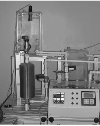
[image:1.612.343.516.320.538.2]systems. The method is applied to a MIMO system where the process outputs are pressure in a tank and liquid level in a connected container. Least-squares method was utilized to determine the parameter estimates. The method is implemented on a desktop PC computer equipped with a data acquisition board. An interface tool was developed for capturing and processing the data. The method can be utilized for parameter estimation of a class of MIMO systems, where prior knowledge of the form of dynamical relations between the inputs and outputs exist.
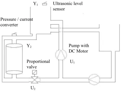
Fig. 2 Block diagram of the pressure-level system
II. IDENTIFICATION OF THE PRESSURE-LEVEL SYSTEM BY THE REAL-TIME PARAMETER
ESTIMATION METHOD
An experimental method is proposed for modeling of the pressure-level system. A black-box model along with a curve fitting approach was used to identify the input-output behavior of the system [2,5].The pressure-level system has two inputs and two outputs.
The inputs to the system are,
U1: control signal applied to the pump,
U2: control signal applied to proportional valve.
The outputs are
Y1: liquid level output signal,
Y2: pressure value output signal.
The following 2x2 system transfer function matrix is obtained
Y1(s) = G11(s).U1(s) + G12(s).U2(s) (1)
Y2(s) = G21(s).U1(s) + G22(s).U2(s) (2)
[image:2.612.64.553.120.699.2]The input-output relation of the system is shown in Fig.3.
Fig. 3 Input-output model of the system
G11 is a transfer function showing the relation between input 1 and output 1. Likewise, G12(s) is the transfer function that shows the effect of input 2 to output 1, G21(s) indicates the effect of input 1 to output 2, and G22(s) indicates the effect of input 2 to output 2.
Initially, a first order transfer function 1 +
s K
τ
is chosen for each input-output relation Gij(s). To find G11(s), an input U2=0 is applied and the relation between input1 (U1) and output1 (Y1) is found.Y1(s)=
(
)
1
U
1s
s
K
+
τ
(3)In this equation, for calculating K and τ constants denominators are equalized and constants are left.
Y1(s).τs+Y1(s)=K.U1(s) (4)
S s U s s Y K s Y K ) ( ) ( 1 )
( 1 1
1 + =
τ
(5)
Transforming the expression from s-domain to t-domain, the 1/s term is converted to an integrator. Equation for Y1
∫
∫
=+ y t dt u t dt K
t y
K () ( )
1 )
( 1 1
1
τ
(6)
1 1 1
1
y (t)
y (t)dt
y (t)dt
K
K
τ
= −
+
∫
∫
(7)dt
t
u
K
dt
t
y
t
y
1(
)
=
−
1
∫
1(
)
+
∫
1(
)
τ
τ
(8)Let’s define the regressors
)
(
)
(
11
t
dt
t
y
=
φ
∫
(9))
(
)
(
21
t
dt
t
u
=
φ
∫
(10)⎭
⎬
⎫
⎩
⎨
⎧
⎥⎦
⎤
⎢⎣
⎡−
=
2 11
)
(
φ
φ
τ
τ
K
t
y
(11)θ
τ
τ
⎥⎦
=
⎤
⎢⎣
⎡−
1
K
(12)
The output equation can be obtained as below
φ
θ
.
=
Y
(13)The regression vector is
( )
φ
Tφ
φ
TY
θ
−1=
(14)+
+ +
Y1(s)
Y2(s)
U1(s)
U2(s)
G11(s)
G12(s)
G21(s)
G22(s)
+
Ultrasonic level sensor Pressure / current
Same calculations are also used for G12(s), G21(s), and G22(s). Calculation of system transfer function parameters are not done in real-time. A MATLAB program is used for this operation.
III. INTERFACED USED FOR REAL-TIME SYSTEM MODELING
[image:3.612.322.537.430.685.2]An interface is designed for calculating the transfer function parameters of the experimental system by the least-squares (LS) method. MATLAB Simulink Real-Time Windows Target Toolbox (RTW) is used for the interface program (Fig.4). Besides, a data acquisition board (NI-DAQ PCI-6024E) is utilized for recording and processing the data. When the interface software runs, signals are applied to system inputs. System outputs are recorded and calculations to determine system parameters are done during run-time.
Fig. 4 MATLAB interface for real-time system modeling
The procedure to identify the transfer functions’ are described as follows:
To find G11(s):
• U2 control input is initialized (zero volt is applied to the proportional valve input),
• U1 control signal is set to several different values (several different voltages are applied to the pump),
• Y1 output (liquid level in the tank) is measured.
To find G22(s):
• U1 control input is initialized (zero volt is applied to the pump),
• U2 control signal is set to several different values (several different voltages are applied to proportional valve),
• Y2 output (pressure in the tank) is measured.
To find G12(s):
• U1 control input is initialized (zero volt is applied to the pump),
• U2 control signal is set to several different values (several different voltages are applied to proportional valve),
• Y1 output (liquid level in the tank) is measured.
To find G21(s):
• U2 control input is initialized (zero volt is applied to the proportional valve input),
• U1 control signal is set to several different values (several different voltages are applied to the pump),
• Y2 output (pressure in the tank) is measured.
Here φ and Y values are recorded. θ is found as
1 K
⎡
−
⎤
= θ
⎢
τ
τ
⎥
⎣
⎦
(15)By using this equation, parameters of Gij transfer function are calculated. At the end of the experiments, elements of system’s transfer function matrix are found as below.
⎥ ⎦ ⎤ ⎢
⎣ ⎡ =
22 21
12 11 ) (
G G
G G s
G (16)
1 s 78.7401616.97638
11= +
G (17)
1 s 24.096394.30343
12 = +
G (18)
1 s 232.5582.1395
21= +
G (19)
1 s 2.4265959.995875
22= +
G (20)
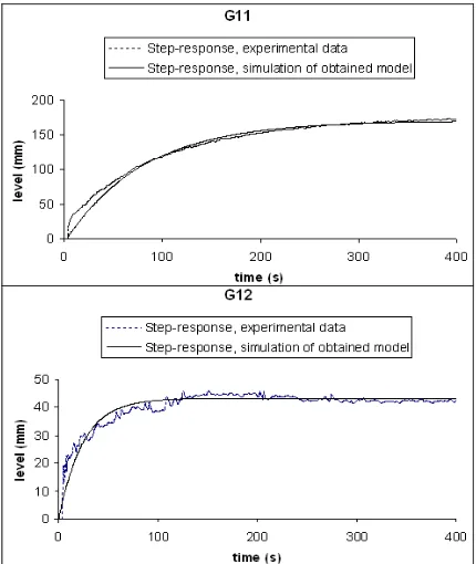
Fig.5 Comparison of experimental step-responses and transfer functions obtained by real-time identification
As shown in Fig. 5, G11, G12, and G22 transfer functions that are found by parameter estimation are fairly close to real system attitude. G21 transfer function does not reflect the real system’s attitude. Because, the real system dynamics is not of a first order dynamics and it is a nonminimum phase system. Thus, G21 transfer function is chosen as indicated.
1 cs bs
k as
-2 21= ++ +
G (21)
Then, parameters are re-calculated after adding an integrator to the interface in MATLAB. The new transfer function for G21, which express the relation between the input U1 and the output Y2 is found.
1 106.193s 141.2236s
98 . 0 57.1756s
-2
21= + + +
G (22)
Simulated step-response obtained from G21 is compared to experimental step-response. Results indicate that the simulation and experimental results follow very closely each other (Fig. 6).
G21
-6 -1 4 9 14
0 100 200 300 400
time (s)
p
res
su
re (
b
ar
)
Step-response, experimental data Step-response, simulation of obtained model
Fig.6 Comparison of G21 simulated step-response with the experimental result.
System’s transfer function matrix is found as below
⎥ ⎥ ⎥
⎦ ⎤
⎢ ⎢ ⎢
⎣ ⎡
+ +
+
++ +
=
1 s 2.4265959.995875 1
106.193s 2
141.2236s
98 . 0 57.1756s
- 24.09639s 1
4.30343 1
s 78.7401616.97638 )
(s
G (23)
For comparison of the identified model with the real system, a MATLAB/Simulink model is formed and tested under various inputs. Fig.7. shows the responses of the system to unit-step applied at both system inputs. Results indicate that the proposed real-time identification method can capture the dynamic behavior of the experimental pressure-liquid level control system successfully.
0 50 100 150 200
0 100 200 300 400
time(s)
level(m
)-P
ressu
re
(b
ar
)
Step-response, experimental data(level) Step-response, experimental data(pressure) Step-response, simulation of obtained model(level) Step-response, simulation of obtained model(pressure)
Fig.7. Comparison of simulated system models and experimental unit-step responses
IV. CONCLUSIONS
REFERENCES
[1] Åström, K.J., Wittenmark, B. (1997). Computer-Controlled Systems. 3rd
ed., pp. 509-514, Prentice Hall.
[2] Kenné G., Ahmed-Ali T., Lamnabhi-Lagarrigue F. and Nkwawo H. (2006). Nonlinear Systems Parameters Estimation Using Radial Basis Function Network. Control Engineering Practice, Volume 14, Issue 7, pp. 819-832.
[3] Mathew A, Athimoottil V., Fairman, Frederick W. (1974). Transfer Function Matrix Identification. IEEE Transactions on Circuits and Systems, v CAS-21, n 5, pp. 584-588.
[4] Perry, R. J., Sun, H. H., Berger W. A. (1998). Determination of a Transfer Function Matrix in Multivariable Systems. IEEE Transactions on Automatic Control, v 33, n 3, pp. 305-307.
[5] Sinha N. K. and Kwong Y. H. (1979). Recursive Estimation of the Parameters of Linear Multivariable Systems. Automatica, Volume 15, Issue 4, pp. 471-475.
[6] Zheng, W.X. (1999). Least-Squares Identification of a Class of Multivariable Systems with Correlated Disturbances. Journal of the Franklin Institute, v 336, pp. 1309-1324.