Abstract—Images have been readily acquired through prevalent, available digital cameras. We could identify and differentiate each image from other ones because of our recognition and past experiences. A computer, on the other hand, has to be trained so that it could recognize things and infer from rules and facts. Ability in recognition of the computer at our level could be a few decades away if not longer. This paper, therefore, proposes an approach to extract structural contents of the image and represent them in efficient forms of B-splines and directional chain codes. Image is first segmented into bounded regions whose boundaries are then approximated by the B-splines. Control points of those B-splines are used to approximate elliptical representations of the regions. In addition, the Chaikin’s algorithm is recursively applied to the control points a few times in order to get more accurate directional chain codes, which could later be used to represent and compared to their counterparts of other images. Consequently, these extracted features could be used for representation, comparison, and retrieval. Moreover, we could use these features to train the computer for recognizing and differentiating images in hope that it would have a cognitive capability comparatively close to us.
Index Terms—B-spline, chain code, image content, structural image representation.
I. INTRODUCTION
A number of images are added into the Internet daily because they are easily obtained and shared. Most search engines, such as Yahoo!, MSN Live Search, and Google, provide image search capabilities. Those image search engines are based on textual and labeling information, and they seem to work fine for the time being. Nonetheless, with an ever increasing number of available images and powerful computing power, those text-based image searches may not be enough to fully deliver more intelligent results to more demanding users. We, therefore, propose an approach that deals with the image contents at the structural level.
Manuscript received December 12, 2007. This work was supported in part by the National Science and Technology Development Agency (NSTDA) of Thailand under Grant F-31-205-20-01 and the King Mongkut’s University of Technology Thonburi (KMUTT)’s Research and Intellectual Property Promotion Center (RIPPC).
Dr. P. Mongkolnam is with School of Information Technology, King Mongkut’s University of Technology Thonburi, Tungkru, Bangkok 10140 Thailand (phone: +662-470-9892; fax: +662-872-7145; e-mail: [email protected]).
T. Dechsakulthorn is a research assistant working under Grant F-31-205-20-01 for School of Information Technology, King Mongkut’s University of Technology Thonburi, Tungkru, Bangkok 10140 Thailand (e-mail: [email protected]).
Asst. Prof. Dr. C. Nukoolkit is with School of Information Technology, King Mongkut’s University of Technology Thonburi, Tungkru, Bangkok 10140 Thailand (e-mail: [email protected]).
Instead of using a text, texture, or color information, we chose to focus on the structures which could be extracted out from the image because they are less dependent or influenced by other factors, such as different lightings, colors, and textures. We begin by segmenting the image based on the image’s pixel information. The neighboring pixels with similar color information are grouped together and then extracted to form regions. The better the segmentation algorithm is used, the better the resulting segmented regions are obtained. We need to be concerned with the chosen algorithm because the structural representations that would be done afterward are rather sensitive to the goodness of the segmented regions. After getting the segmented regions, we use the B-splines [1] to approximate the regions’ boundaries. Ideally, the B-splines should be used to represent the extracted structures; however, to speed up a comparison time, the coarser representations could be used instead.
The coarser representations are ellipses and directional chain codes. Each region’s ellipse is obtained by approximating a convex hull of each control polygon of the B-spline. The control polygon is obtained by connecting the control points. The directional chain codes [2] are obtained by considering the eight possible directions (from 0 to 7 as corresponding to the geographical E, NE, N, NW, W, SW, S, and SE) of each control polygon’s segment. To improve accuracy of those directions, the control polygon needs to be refined by being applied to the Chaikin’s corner-cutting algorithm [3] a few times.
For the rest of this paper, we first give some background and related work on image analysis, representation and retrieval. Next, our work on extracting and representing structural image content is given. Last, the conclusion and future work are presented.
II. RELATED WORK
Much work has been done on image analyses in the last few decades. The work traditionally applies image-processing techniques to still images and videos. Image information, such as color and texture, has been the basis for those techniques. Later work has included two-dimensional shapes in its analyses, but the shape analyses have been limited to profiles of objects, such as fish, handwritings, and airplanes. F. S. Cohen, Z. Huang, and Z. Yang [4] use B-splines to model curves for those objects’ silhouettes. The curves are used to identify object’s shapes and match them against others for retrieval. In matching and classifying the curves, they use two methods: the control point-based method and residual error-based method. Similarly, Y. Wang and E. K. Teoh [5] use B-splines and their curvature property, the curvature scale space (CSS) image, to model and match shapes. The CSS image is
Extracting Structural Image Contents
constructed by convolving the smoothened curve with a Gaussian function at different scale levels, and using the locations of the inflection points of the resulting curves for shape matching.
H. Nishida [6] uses directional chain codes for indexing structural features in his image shape retrieval. His image database includes a collection of the already, clearly extracted boundary contours of marine creatures and plant leaves. Each boundary is a closed, polygonal approximated contour. His method is based on indexing structural features and ranking model images, using a voting technique that compares them to extracted features from the query image. A. Del Bimbo and P. Pala [7] propose a shape indexing using a multi-scale representation, which is more robust than other work that works on a single-scale analysis. The key, characterizing shape elements are preserved whereas other details are progressively screened out. The graph structure is used to represent shape parts at different levels. To search shapes in a database that are similar to structural parts of a query shape, the graph is traversed from a coarse to fine level. In other shape matching work, T. B. Sebastian and B. B. Kimia [8], and H. Sundar, D. Silver, N. Gagvani, and S. Dickinson [9] use medial axis or skeletal graphs for representing and matching both two-dimensional and three-dimensional shapes’ interiors. The medial axis graphs overcome some fundamental shortcomings of the outline curves whose internal structures are not known.
A thorough discussion on shape analyses for image retrieval could be found in the work of D. Zhang and G. Lu [10], and a good overview on using shapes in content-based image retrieval is given in [11], [12] as well.
III. METHODOLOGY
We start segmenting an image into regions according to its pixel color information. We choose the JSEG algorithm developed by Y. Deng, B. S. Manjunath, and H. Shin [13] due to its capability to automatically segment the image and provide good segmentation of many color images. The algorithm consists of both color quantization and spatial segmentation, using a multi-scale region growing method. The boundaries of the segmented regions are then approximated and represented by the parametric B-splines. We use the B-splines because of its compact representation, its smooth approximation, and its local control and low-degree property. The B-spline curve, C(u), is defined as:
∑
= = h i i p , i (u)P N ) u ( C 0 (1) where p is a degree, Pi is a control point, u is a parameter, andNi, p is a B-spline basis function, which is recursively defined
as:
≤ <
= + otherwise 0 if 1 1
0 i i
,
i (u) u u u
N ) u ( N u u u u ) u ( N u u u u ) u ( N p , i i p i p i p , i i p i i p , i 1 1 1 1 1 1 − + + + + + + − + − − + − − = (2)
where ui is a knot, the joining point of two curves’ segments.
In order to approximate a region’s contour, the curve is not intended to pass through all the sampled data points of the contour. To measure how close an approximation of the curve to the data points is, a sum of square distance error is computed. The distance error is measured as a distance between each sampled data point and its corresponding point on the approximating curve. Our goal is to get a good enough approximation by trying to minimize the summed square distance error. The approximation can be summarized as: Input: A set of n+1 contour’s sampled data points, D0, … ,
Dn.
Output: The degree p B-spline curve with h+1 control points, P0, … , Ph that meets the following two conditions.
First, the curve must pass through the first and last sampled data point. Second, the curve approximates the sampled data points in a sense of a least square distance error.
Due to the first condition, the resulting curve equation is now defined as:
( )
( )
n p , hh
i i,p i p , D u N P ) u ( N D u N ) u ( C + + = ′
∑
− = 1 1 00 (3)
Now, let the n+1 curve’s parameters be t0, …, tn. Note that the
number of the parameters is equal to the number of the sampled data points because there must be a corresponding point on the curve at each parameter for each sampled data point on the contour as previously mentioned. There are many ways to compute the parameters, but we choose the centripetal parameterization due to its effectiveness. It is computed as:
2 1
1 1
∆ ∆ = ∆ ∆ + + i i i i x x (4) where ∆i is ti+1−ti, and ∆xi is Di+1−Di. And the sum of all
square distance errors is computed as:
(
)
∑
−( )
= − = − 1 1 2 1 1 nk k k
h D C t
P , , P
f K (5)
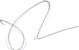
[image:2.595.364.502.647.735.2]We strive for a minimum of the objective function, f(.), given in (5) in order to obtain good control points of the approximating B-spline curve. After getting the control points, we use (1) to generate the B-spline curve. Fig. 1 shows a coarse B-spline curve approximation to the test data points. Here, we show an open-ended curve approximation where the first data point is not the same point as the last data point. This B-spline curve has degree three and ten control points. A higher number of the control points would result in a closer approximation than the one shown here.
We want to represent each structure in a multiscaling setting, from a coarse to fine level-of-detail. First, the coarsest representation is an ellipse. The next one is a control polygon, which is obtained from the control points. The next finer ones are the Chaikin’s corner-cut polygons; two levels of applying the Chaikin’s algorithm suffice for our work. Last, the finest one is the B-spline curve itself.
Ellipses are chosen as the coarsest representation because they could effectively represent most structural shapes comparatively to other geometric figures, such as rectangle and polygon. Ellipse is compactly represented by its origin, semi-minor axis, and semi-major axis. Its orientation is along the major axis. Larger ellipse is rendered behind smaller ellipses to give us a sense of viewing distance. Fig. 4(d), Fig. 5(d), Fig. 6(d), and Fig. 7(d) show elliptical representation of the original images.
The control polygon is obtained by sequentially connecting control points. Fig. 4(e), Fig. 5(e), Fig. 6(e), and Fig. 7(e) show the obtained control polygons of the approximating B-spline curves. A finer representation is the Chaikin’s corner-cut polygon. The algorithm is defined as: Given a control polygon, {P0, … , Pn}, a new set of refined
control points is {Q0, R0, Q1, R1, … , Qn-1, Rn-1}, where each
new pair of points Qi, Ri is computed to be at ¼ and ¾ of a
line segment PiPi+1. The new refined polygon could be recursively used as input for the next, finer level. Fig. 2 illustrates the Chaikin’s corner-cutting sequence. The more times the Chaikin’s algorithm applies to a curve, the smoother the resulting curve and the closer the approximation is. Theoretically, if we apply the Chaikin’s algorithm to the limit, the resulting curve would be a quadratic B-spline. In practice, however, applying the algorithm a few times already results in a good approximation.
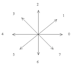
For the most precise representation, we use the B-spline curve because of its relatively more accuracy. Fig. 4(c), Fig. 5(c), Fig. 6(c), and Fig. 7(c) show the approximating B-spline curves. To do a curve matching, a curvature is used for comparison as done in [5]. In order to reduce complexity of using the curvature, we instead use the directional chain codes to represent the curve. The directions of the chain codes are a set of directions of polygon legs of the Chaikin’s corner-cut polygon. The possible eight directions used are shown in Fig. 3.
[image:3.595.367.484.51.156.2](a) (b) (c) Fig. 2: Chaikin’s corner-cut polygons. (a) Control polygon. (b) First-level corner-cut polygon. (c) Second-level
corner-cut polygon.
Fig. 3: Eight directional chain codes.
If the directional chain codes were used to represent the triangle’s control polygon of the test image, in Fig. 4(e), we would get the codes as follows:
Direction Length Level 0 4.14 4 6 17.69 2 7 113.53 0 4 76.61 0 2 112.27 0
Direction could be one of the eight possible vectors shown in Fig. 3. In the code above, a sequence of directional vectors consists of vector 0, 6, 7, 4, and 2 in a clockwise manner. Length represents magnitude of each vector. Level indicates the relative significance of each vector to other vectors with respect to the total length of the control polygon. There are five total levels, from 0 to 5 with level 0 being the most significance. If the vector’s magnitude is ≥ 20% of the total length, it will be at level 0; if ≥ 10%, it will be at level 1; if ≥
5%, it will be at level 2; if ≥ 2.5%, it will be at level 3; if ≥
1%, it will be at level 4; the other will be at level 5. From the above chain codes, the vector 7, 4, and 2 are at the most significant level, and they collectively represent the triangle, when considered in a clockwise direction.
Likewise, the directional chain codes for the square’s control polygon would be as follows:
Direction Length Level 1 11.62 3 7 14.25 2 0 40.64 1 6 58.92 0 5 18.38 2 4 60.73 0 2 64.35 0
Here, you can see a problem arises in that there is a sequence of directional vector 6, 4, and 2, when considered at the most significant level 0. The missing vector 0 is mistakenly placed at level 1 instead of level 0 due to the coarse nature of the control polygon.
In order to get a more accurate chain code representation, we apply the Chaikin’s corner-cutting algorithm to each control polygon. Applying the algorithm twice empirically results in the good, finer control polygons. Thereafter we compute for the corresponding directional chain codes. Now, the codes for the square are:
[image:3.595.53.283.608.739.2]7 4.82 4 6 55.46 0 5 9.35 3 4 54.99 0 3 4.82 4 2 53.89 0
The codes have a more correct sequence of directional vectors, that is, the vector 0, 6, 4, and 2, when considered at the most significant level 0. Moreover, the magnitude of each vector is not much different from the others. Better results are obtained for other structures, such as octagon, triangle, and rectangle as well.
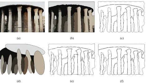
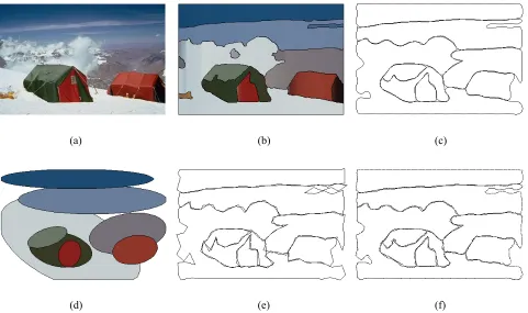
We also apply our method to the real images in Fig. 5, Fig. 6, and Fig. 7. The structures of columns, dinosaur, and tents seem to be satisfactorily extracted and represented. For instance, the middle column of Fig. 5 is represented by the following codes.
Direction Length Level 1 14.22 3 0 26.76 2 7 3.46 5 6 208.02 0 5 3.81 5 4 27.84 2 3 7.16 4 2 200.23 0
It is obvious that vector 6 and vector 2 are the most significance, and vector 0 and vector 4 are the second most one. Consequently, a sequence of the directional vector 0, 6, 4, and 2 represents somewhat a rectangular structure in the image.
IV. CONCLUSION
We have illustrated the approach to analyze the image contents by extracting the structures out and representing them using the ellipses, B-splines, and directional chain codes. The B-splines are chosen to represent the boundaries of the extracted regions because of their compact representation and effective approximation nature. In addition to using the B-spline representation, the elliptical representation and the directional chain code representation are used as additional features. The B-splines’ control points are used to get both the elliptical representation and the directional chain code representation. The obtained directional chain codes may not correctly represent the structural shape unless the control points are refined further by being applied to the Chaikin’s corner-cutting algorithm.
This work is merely a beginning of what the future work in image analysis, image understanding, and image comparison would be like. When the image could be segmented into more meaningful structures, or when the foreground objects are correctly extracted out of a background, and thus the structural comparison would become indispensable for the object recognition of any intelligent systems.
V. FUTURE WORK
An improvement on the image segmentation is vital to the subsequent processes. The segmentation technique does not work perfectly when the color differences are not substantial enough for the algorithm to correctly segment the image. When a near perfect segmentation is obtained, our structural image representation would dramatically improve the image comparison and retrieval due to the desired image structural content information. Curve comparison could be used in place of the chain code comparison as done here for curvy, smooth structures. An improvement on the chain code representation and its comparison algorithm is also needed for a faster and more efficient comparison. Furthermore, a two-dimensional curve representation could be extended to a three-dimensional one in a three-dimensional object comparison and retrieval.
ACKNOWLEDGMENT
The work is partially supported by the National Science and Technology Development Agency (NSTDA) of Thailand under grant F-31-205-20-01 and the King Mongkut’s University of Technology Thonburi (KMUTT)’s Research and Intellectual Property Promotion Center (RIPPC). The last three images are by courtesy of J. Z. Wang at Penn State.
REFERENCES
[1] G. E. Farin, “Curves and Surfaces for CAGD: A Practical Guide,” Morgan Kaufmann, 5th edition, Oct. 2001.
[2] S. Junding and W. Xiaosheng, “Chain code distribution-based image retrieval,” Proceedings of the 2006 International Conference on Intelligent Information Hiding and Multimedia Signal Processing (IIH-MSP’06), 2006.
[3] G. Chaikin, “An algorithm for high speed curve generation,” Computer graphics and image processing, pp. 346-349, 1974.
[4] F. S. Cohen, Z. Huang, and Z. Yang, “Invariant matching and identification of curves using B-splines curve representation,” IEEE Transactions on Image Processing, vol. 4, no. 1, pp. 1-10, Jan. 1995. [5] Y. Wang and E. K. Teoh, “2D affine-invariant contour matching using
B-spline model,”IEEE Transactions on Pattern Analysis and Machine Intelligence, vol. 29, no. 10, pp. 1853-1858, Oct. 2007.
[6] H. Nishida, “Shape retrieval from image databases through structural feature indexing,” Vision Interface ’99, Trois-Rivieres, Canada, pp. 328-335, May 1999.
[7] A. Del Bimbo and P. Pala, “Shape indexing by multi-scale representation,” Image and Vision Computing, vol. 17, nos. 3-4, pp. 245-261, 1999.
[8] T. B. Sebastian and B. B. Kimia, “Curves vs. skeletons in object recognition,” International Conference on Image Processing, 2001. Proceedings, vol. 3, pp. 22-25, Oct. 2001.
[9] H. Sundar, D. Silver, N. Gagvani, and S. Dickinson, “Skeleton based shape matching and retrieval,” Shape Modeling International, pp. 130-139, May 2003.
[10] D. Zhang and G. Lu, “Review of shape representation and description techniques,” Pattern Recognition, 37(1), pp. 1-19, 2004.
[11] A. W. M Smeulders, M. Worring, S. Santini, A. Gupta, and R. Jain, “Content-based image retrieval at the end of the early years,” IEEE Transactions on Pattern Analysis and Machine Intelligence, vol. 22, no. 12, pp. 1349-1380, Dec. 2000.
[12] J. Z. Wang, J. Li, and G. Wiederhold, “SIMPLIcity: semantics sensitive integrated matching for picture libraries,” IEEE Transactions on Pattern Analysis and Machine Intelligence, vol. 23, no. 9, pp. 947-963, Sep. 2001.
[13] Y. Deng, B. S. Manjunath, and H. Shin, “Color image segmentation,”
(a) (b) (c)
[image:5.595.57.531.70.326.2]
(d) (e) (f)
Fig. 4: Test image and its extracted structures. (a) Original test image. (b) Segmented image. (c) B-spline curve approximation to structural contours. (d) Elliptical approximation. (e) B-splines’ control polygons. (f) Directional chain code representation
of the B-splines’ control polygons.
(a) (b) (c)
(d) (e) (f)
Fig. 5: Image and its extracted structures. (a) Original image. (b) Segmented image. (c) B-spline curve approximation to structural contours. (d) Elliptical approximation. (e) B-splines’ control polygons. (f) Directional chain code representation of
[image:5.595.63.533.427.694.2](a) (b) (c)
[image:6.595.54.533.63.346.2](d) (e) (f)
Fig. 6: Image and its extracted structures. (a) Original image. (b) Segmented image. (c) B-spline curve approximation to structural contours. (d) Elliptical approximation. (e) B-splines’ control polygons. (f) Directional chain code representation of
the B-splines’ control polygons.
(a) (b) (c)
(d) (e) (f)
Fig. 7: Image and its extracted structures. (a) Original image. (b) Segmented image. (c) B-spline curve approximation to structural contours. (d) Elliptical approximation. (e) B-splines’ control polygons. (f) Directional chain code representation of
[image:6.595.54.535.436.721.2]