Job Mobility in Ireland
ADELE BERGIN*
National University of Ireland Maynooth and Economic and Social Research Institute, Dublin
Abstract:This paper investigates the factors that determine job-to-job mobility in Ireland over the period 1995 to 2001. It finds that labour market experience, working in the public sector, whether a person is overskilled, the sector they work in and their occupation are important determinants of voluntary job change. The paper finds the rate of voluntary job mobility in Ireland trebled over the period 1995 to 2000. The sample is divided into two time periods and a decomposition technique is applied to ascertain how much of the increase in mobility is attributable to compositional changes and how much is due to other factors. Compositional changes explain around one-third of the increase, while the remainder seems to reflect fundamental changes in the operation of the labour market.
I INTRODUCTION
T
he focus of this paper is to investigate the various factors that determine job-to-job mobility in Ireland. The dataset used covers most of the Celtic Tiger period, a time where growth in the Irish economy was exceptional, and the paper addresses the effect the changing labour market had on job mobility. Job mobility1 is an important phenomenon to understand because the movement of workers from one job to another allows for flexibility in the labour market by providing workers and firms with a mechanism to adapt to15
*The author would like to thank Aedin Doris, Donal O’Neill, Olive Sweetman, seminar participants at the 2008 Irish Economic Association Conference and the NUIM PhD Seminar Group for helpful comments and suggestions.
1Job mobility refers to the ability of workers to change jobs; in practice realised job changes are used as a proxy for job mobility.
changing economic and personal circumstances. It is a process that allows for and promotes allocative efficiency in the labour market.
Over the course of the 1990s the Irish economy experienced spectacular growth rates with GNP growth averaging 7.9 per cent per annum over the period 1995 to 2001. The success of the Irish economy over this period was built on factors that affected labour supply, such as the favourable demographic structure of the labour force, a dramatic rise in female participation rates and net immigration, particularly towards the end of the period, and factors that affected the demand for labour such as foreign direct investment and competitiveness. Over this period, labour supply growth averaged 3.4 per cent per annum and employment increased by an average of 67,000 per annum (on a PES basis), implying that the number of jobs created over the period far exceeded the number of jobs that were destroyed. Existing research tells us that some of these jobs were filled by those returning to the labour market, particularly women (see Doris, 2001), and immigrants or returning nationals (see Barrett, Fitz Gerald and Nolan, 2002). However, little is known about existing workers who changed jobs over the period as well as what affected their decision to do so and this paper seeks to bridge that gap.
One of the findings of the paper is that the rate of voluntary job mobility trebled over the period 1995 to 2000. The paper also investigates the potential causes of this increase – is it simply driven by changes in the composition of workers or do other factors such as changes in the labour market conditions facing workers play a role?
The paper is organised as follows: Section II surveys the theoretical literature on job mobility and outlines what the literature tells us we should observe in the data, Section III describes the dataset, the construction of key variables and provides some descriptive statistics. Section IV presents the results of some multinomial probit models of job change and how we take account of changes in the labour market environment over the period. Section V outlines a decomposition technique that is used to ascertain the extent to which the increase in mobility is driven by changes in the composition of the sample. Section VI concludes.
II BACKGROUND
2.1 Why do Workers Change Jobs? Theoretical Models
In these models the labour market is typically characterised by imperfect information or by some degree of heterogeneity. It is usually assumed that there is a range of different jobs in the labour market and that individual workers differ in their ability to perform the tasks associated with any of these jobs. In other models, the assumption of imperfect information means that firms are uncertain about the productivity of a worker at the beginning of an employment relationship. As a result, workers may not be initially employed in the jobs in which they are the most productive. Job mobility provides a mechanism for the labour market to move towards a more efficient allocation of resources whereby workers sort themselves into jobs that maximise their productivity. Three main theoretical approaches can be distinguished from the literature, namely job search models, job matching models and human capital models.
At the core of job matching models is the idea that the labour market is characterised by imperfect information. In Jovanovic’s (1979) seminal contribution, the quality of an employment match, where quality is defined in terms of the worker’s actual productivity in a particular job, is not known ex ante. Over time, as tenure increases, information about the worker’s productivity is revealed and prior expectations about the quality of the match are updated. This information leads to either job continuance or job turnover when the quality of the match is worse than initially expected. Consequently, the probability of mobility declines with tenure. Workers move to increasingly higher quality matches, where they are rewarded more for their particular aptitudes. This model predicts a positive relationship between job mobility and wages, although it is not a direct relationship but rather wages are affected through improved match quality.
Human capital models (such as Becker (1962) and Oi (1962)) imply an inverse relationship between job mobility and investment in job-specific skills, which incorporates both on-the-job experience and any formal training. As tenure in a job increases, workers acquire more specific human capital and this creates a higher earnings potential for that person in their job, and so reduces the probability of job mobility. The nature of the human capital a worker acquires on-the-job, in particular its transferability to another job, will determine the wage impact of changing jobs. If specific human capital is an important determinant of earnings, changing jobs may result in wage losses.
Many modern theoretical models build on the models described above. However, there are alternative approaches. Blumen et al. (1955) was one of the first models of job mobility. In their mover-stayers model, workers have an unobservable characteristic such as the capacity to stay in a job, that affects their productivity. High productivity workers will avoid job turnover, while low productivity workers will change jobs frequently. In this model, mobility is negatively correlated with wages because it is correlated with the unobservable characteristic that determines mobility. In direct contrast, in Lazear’s (1986) raiding model, mobility acts as a positive signal of productivity and leads to wage gains. In this model, firms use workers’ previous wages as an indicator of their quality and so high productivity workers’ experience more mobility than low productivity workers because the highest paying firms poach workers from their rivals.
2.2 Patterns We Should Observe in the Data
(a) Labour Market Conditions
Turnover rates should vary over the course of the business cycle. During upturns there is an increase in vacancies and so there are more potential employment opportunities available to workers. In job search models, this would lead to an increase in the job arrival rate. In job matching models there is an increase in the number of alternative jobs a worker can switch to. In general, we would expect workers to have a higher probability of quitting when they have a good chance of obtaining a better job quickly. Therefore, when labour market conditions are tight we would expect to see more quits then when they are loose (see for example, Hamermesh (1996)). Conversely, layoff rates tend to be anti-cyclical; when demand falls employers will layoff workers.
whose productivity is unknown and this may lead to higher subsequent job separations. Similarly, downturns in activity provide employers with an opportunity to shed their least productive workers, thus reducing the need for subsequent adjustments in their workforce.
(b) Effects of Tenure, Age and Experience
Age is an important factor determining job mobility and turnover declines with age. In Stigler (1962) younger workers are more likely to try a variety of jobs in order to acquire knowledge of the labour market and their own preferences and ability for different jobs (a process known as “job shopping”) so we should expect to see higher mobility rates for younger workers. As workers gain labour market experience, they move to better job matches. In job search models, with each job change the worker moves up the wage offer distribution leaving them with fewer jobs to which it would be worthwhile for them to move to in the future so mobility declines with experience. This is supported empirically by numerous studies. For example, Topel and Ward (1992) find that for young men two-thirds of their total lifetime job mobility occurs within the first ten years of their career. They see job mobility for young workers as a crucial phase in workers’ movement to more long-term stable employment relationships.
exceed the costs. If the gains involved in changing jobs put a worker on a higher wage path younger workers will benefit for longer from these gains. In addition, older workers may have higher time preferences and therefore apply a higher discount rate on future earnings so job mobility declines with age.2
(c) Gender
Central to why we might expect differential mobility rates by gender is that women have a lower attachment to the labour force. Barron et al. (1993) develop a job-matching model where workers differ in their attachment to the labour force. The model predicts that those with a weaker attachment to the labour force are sorted into jobs that offer less training and that use less capital and as a result have less to lose by changing jobs in terms of specific capital. On the other hand, women may be less likely to change jobs if they are more constrained by non-market variables such as their partner’s location or the rearing of children (Royalty, 1993). Empirically, several studies have found that by controlling for characteristics, such as labour market experience, gender differences in turnover rates diminish or disappear (e.g. Blau and Kahn, 1981; Loprest, 1992; Booth and Francesconi, 1999).
(d) Education
There are several reasons to expect a relationship between education and job mobility but there is no consensus in the literature as to whether it is positive or negative. On the one hand, the specific human capital model implies that education increases job duration and therefore, reduces mobility. It is also possible that individuals with more specific human capital may be less likely to experience job change, because the specific nature of their human capital may have no value to other employers. Connolly and Gottschalk (2006) observe that less educated workers may invest less in human capital and consequently have less to lose by changing jobs. They will, therefore, have a lower reservation value when approached with an alternative job offer. Weiss (1984) suggests that there is an unobservable characteristic, which he calls “stick-to-itiveness”, that affects both the value of education and the value of staying in an existing job. In addition, Barron et al. (1993) argue that education may qualify workers for high training jobs or capital-intensive jobs and so incentives are offered to decrease the expected number of quits for better-educated workers. Neal (1999) proposes a model of job search that involves both employment matches and career matches. He argues that less
educated workers are likely to experience more job turnover because they experience mobility that involves career change and then they search for a good employment match. Therefore, it is possible that the process of finding a good career match may add considerably to the wage growth of younger workers, especially the less educated. To the extent that better educated workers (especially those with college degrees) use time spent in education as a form of pre-market search, they are less likely to experience mobility that involves career changes.
However, it is also possible that there could be a positive relationship between education and mobility. Weiss (1984) argues that education increases workers alternative opportunities and so may increase job mobility. Johnson (1979) argues that higher wage variance may increase the option value of job mobility, so highly educated workers may experience more job turnover as they face more variable but potentially more rewarding alternative job offers. In addition, Greenwood (1975) contends that highly educated individuals may be more efficient job searchers and so have lower transactions costs and, therefore, may change jobs more easily. It is possible that better educated workers are more likely to have ‘faster’ careers and will change jobs more frequently as a means of advancing up the career ladder (Borsch-Supan, 1987). Finally, Bartel and Lichtenberg (1987) put forward the idea that highly educated workers have a comparative advantage in learning and implement -ing new technologies and so firms may provide incentives to reduce job quits.
III DATASET, DEFINING JOB MOBILITY AND DESCRIPTIVE STATISTICS
3.1 Dataset and Sample Construction
The Living in Ireland Survey (LIS) is used to investigate the determinants of job change. The LIS constitutes the Irish component of the European Community Household Panel (ECHP) which began in 1994 and ended in 2001. It involved an annual survey of a representative sample of private households and individuals aged 16 years and over in each EU member state, based on a standardised questionnaire. A wide range of information on variables such as labour force status, occupation, income and education level is collected. There is also a wealth of data collected on job and firm characteristics.3
To identify those who have changed jobs I make use of the panel dimension of the LIS. A revolving balanced panel of people aged 20 to 60 years, roughly
the prime working age, has been selected from the LIS. The reason for this is that a balanced panel prevents the entry of younger people into the sample and so over time, as the fixed sample ages the proportion of younger people would decline.4Individuals are included in the sample for some years but not for others if they fail to meet the age restriction.5 Each individual’s labour force status is then categorised on a PES basis. Individuals, who are categorised as employed, are those who work or usually work at least 15 hours per week. I only consider cases where labour force status is available in each year they are eligible for inclusion in the sample. In each year there are around 20 people whose labour force status cannot be classified.6These cases are deleted from each year of the sample.
Table 1 shows the total sample size each year and provides some basic characteristics of the sample. The average age of the sample declines over the period implying that the impact of the baby boom generation outweighs the effect of the ageing of the sample. The sample participation rate appears high but it is measured as the proportion of people in the labour force aged 20 to 60 as a percentage of the total number of people age 20 to 60.7 The male participation rate is significantly above that of the female participation rate, however there is a dramatic rise in the female rate over the period. The Table also shows that participation rates decline with age, as we would expect, and that the participation rates for those over the age of 30 increased between 1994 and 2001.8
3.2 Calculation of Job Mobility
To capture job changes we need to be able to identify those who have separated from their employer between waves. The LIS does not contain an explicit question about changing jobs. However, job mobility can be inferred from answers to the question When did you begin work with your present employer (or in your present business)? Please specify the month and the year.
4For example, someone who is aged 20 in 1995 will be 26 years in 2001 and if we only considered the same group of people over time (a balanced panel), there would be no one below the age of 26 years in the panel by 2001. Effectively, a revolving balanced panel allows younger people into the sample in later years.
5This approach to selecting a sample is similar to that of Baker and Solon (1999).
6These individuals are either not working and no reason is given for why they are not seeking work or in the bulk of cases they are in remedial training or sheltered workshops.
7Using CSO data, the participation rate for those aged 15 to 64 years rose from 60 to 66 per cent over the period. This is below the participation rate of the sample given in Table 1, but it considers more younger and older people who are less likely to be in the labour force and so it is at least consistent with the rate given in Table 1.
The response to this question is used to measure workers tenure in their current job. If we observe that an individual was working in the previous year and if their response to this question in the current year is less than the time elapsed between interviews then we conclude that this person has changed jobs.
Job mobility is defined in terms of employment-to-employment transi -tions. To capture this in the data workers need to be employed in two consecutive years. For example, someone who is employed in one year and then unemployed for two years and then employed again is not included in the analysis. Even though this person has changed jobs over the four-year period, they have moved from being employed to being unemployed for two years to being employed again. Restricting the sample to people who are employed in consecutive two-year periods means that this type of case is excluded. I have excluded these types of transitions because the decision to change jobs is different to the decision to move from, say non-participation or unemployment to employment. This definition of job mobility only allows people to be unemployed or to not participate in the labour market for a relatively short amount of time between jobs, essentially less than a year (or more precisely less than the amount of time between interviews). In addition, this measure of job mobility may underestimate total job mobility if more than one job change occurs between subsequent interviews. Farber (1999) states that one of the central facts about job mobility is that there is a high hazard of jobs ending within the first year of an employment relationship.
[image:9.556.66.425.98.248.2]Individuals who are employed in successive two-year periods are selected from the revolving balanced panel. The resulting sample is one with workers who have a high attachment to the labour force. In each year around 12 people do not give a response to the question about how long they have been
Table 1:Revolving Balanced Panel of Individuals Aged 20 to 60 Years
1995 1996 1997 1998 1999 2000 2001
Total Sample Size 2,417 2,367 2,338 2,299 2,294 2,325 2,357 Average Age 42.0 41.8 41.5 41.2 40.9 40.4 40.1
% % % % % % %
with their current employer and they are excluded from the sample. This results in 1,916 people in the analysis and 9,377 person-year observations. Table 2 shows the number of workers employed in consecutive two-year periods and the rate of job change. Each year approximately 10 per cent of workers change jobs. However, this figure masks an important trend evident in the data. In 1995, 6.5 per cent of workers changed jobs and this rate increased over the period so that by 2000 the mobility rate was 13.5 per cent.
Table 2: Job Mobility Rate
1995 1996 1997 1998 1999 2000 2001
Number of workers 1,185 1,229 1,274 1,337 1,406 1,449 1,497 No. Job Changes 77 89 110 146 151 195 159 Job Mobility Rate 6.5% 7.2% 8.6% 10.9% 10.7% 13.5% 10.6%
[image:10.556.72.434.344.433.2]A total of 927 job changes are identified, however, some people changed jobs more than once so Table 3 shows the number of jobs held by the 1,916 workers between the beginning and end of the 7-year period.
Table 3: Number of Job Changes Per Worker
0 1,328
1 375
2 126
3 57
4 21
5 9
To put Ireland in an international context, Table 4 shows average estimates of job mobility for young workers over the period 1995 to 2001 across a range of European countries. From the Table we can see that young workers in Ireland have a relatively high rate of job mobility.9
The LIS also asks the main reason for the previous employment relationship ending. This allows us to identify worker initiated or voluntary quits such as obtaining a better job, family-related quits etc. and employer related or involuntary quits such as redundancy, dismissal, business closure
etc. It may be important to be able to distinguish between voluntary and involuntary job turnover as the reason for job separation is likely to have different impacts on subsequent wage growth.10Table 5 gives the main reason why job changers stopped working in their previous jobs. In each year the bulk of job changes were voluntary, with 50 per cent of job changes being voluntary in 1995 rising to just around 65 per cent in 2001.11 In 1995, 32 per cent of mobility was involuntary and this tended to fall over the period so that by 2001 around 21 per cent of all job changes were involuntary. Unfortunately, around 16 per cent of people who changed jobs over the period did so for another reason that was not included in the questionnaire or they did not answer the question. These workers are excluded from the analysis that follows and Table 6 shows the number of workers employed in consecutive two-year periods and the rate of job change for the resulting sample.
3.3 Descriptive Statistics
[image:11.556.67.425.108.274.2]This section examines some individual characteristics of workers and of those who change jobs. The aims are to identify differences in characteristics between those who change jobs and those who stay in their jobs and also to Table 4: Job Mobility Rates, Average Between 1995-2001 for Workers Under 30
Years in 1994
%
Germany 6
Netherlands 8
Austria 8
Portugal 9
Belgium 10
France 10
Italy 10
Greece 13
Ireland 16
UK 19
Finland 22
Spain 23
Source:Davia (2005), estimates derived from the European Community Household Panel Survey.
10For example, Keith and McWilliams (1999) find differential rates of return to job mobility in the US depending on whether the reason for separation is voluntary or involuntary.
any compositional changes in the total number of workers that might help explain the rise in the rate of voluntary job change.
Age
[image:12.556.73.436.92.361.2]The age distribution of all workers in the sample (from Table 6) is given in Table A1. The proportion of workers in the 20 to 29 year age group increases over time, and the increase is more marked in 2000 and 2001, reflecting the fact that these younger people only have to be working for a relatively short period of time for them to be included in the sample. The proportion of workers in the 30-39 year age group declines over the period, consistent with the ageing of the sample over time. The proportion of the workers in the 40 to 49 year age group increases up to 2000, again indicating the ageing of the sample.12The proportion of workers between 50 and 60 years declines slightly over the period because the impact of people dropping out of the sample at 60 years slightly dominates the effect of ageing. There is a slight decrease in the
Table 5: Reason for Stopping Previous Job
1995 1996 1997 1998 1999 2000 2001
% % % % % % %
Voluntary Turnover:
Got Better Job 47 43 43 42 46 54 57 Other Reasons Given 3 7 10 15 16 12 9
Involuntary Turnover:
Obliged to Stop 10 11 12 16 8 10 9 End of Contract 22 24 15 11 15 11 12
Rest 18 16 20 15 15 12 13
Table 6: Job Mobility Rate
1995 1996 1997 1998 1999 2000 2001
Number of workers 1,171 1,215 1,252 1,315 1,384 1,425 1,476 No. Job Changes 63 75 88 124 129 171 138
% % % % % % %
Overall Job Mobility Rate 5.4 6.2 7.0 9.4 9.3 12.0 9.3 Voluntary Mobility Rate 3.2 3.6 4.6 6.4 6.8 9.1 7.0 Involuntary Mobility Rate 2.1 2.6 2.4 3.0 2.5 2.9 2.3
[image:12.556.75.434.99.227.2]average age of workers over the period due to the impact of the ‘baby boom’ generation.
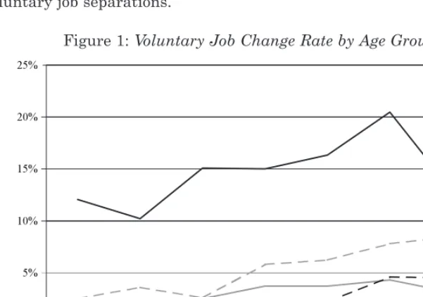
Table A1 also shows the percentage of each age group who experience voluntary and involuntary mobility over time. From the Table we can see that the propensity to voluntarily change jobs declines with age and this finding is consistent with the empirical literature. This relationship is also shown in Figure 1. The increasing proportion of young people aged 20 to 29 years is, at least in part, driving the increase in the overall mobility rate. Interestingly, the mobility rates for workers over the age of 30, although somewhat volatile over the period, show quite large increases. For example, the rate of job change for those between 30 and 39 almost trebles over the period, albeit from a much lower base than comparable rates for workers aged between 20 and 29 years. Workers who change jobs are on average 8/9 years younger than the sample average. The rates of involuntary change by age group are closer together, although those in the 20 to 29 year age category experience the highest rate of involuntary job separations.
Gender
[image:13.556.96.397.314.525.2]Table A2 shows the gender distribution of workers over time. Female workers account for a rising proportion of workers over time capturing female workers who returned to the labour market. The percentage of men and women who change jobs by type of change is also given in Table A2. Female workers experience a higher rate of voluntary mobility than male workers and
male workers experience a higher rate of involuntary mobility. Both the male and female rates of voluntary job mobility increase over the period 1995 to 2000 with the female rate increasing at a faster pace. The female voluntary job change rate is around 1 percentage point above the male rate so the changing gender distribution of workers may be contributing somewhat to the rise in the voluntary job mobility rate over the period.
Education
Table A3 shows the education distribution of all workers where low-skilled workers are those who have, at most, Junior Certificate education, medium-skilled are those who have, at most, a diploma and high-medium-skilled are those with degrees.13From the Table, an improvement in the educational attainment of workers is apparent with low-skilled workers accounting for a declining proportion of the total and medium- and high-skilled workers accounting for an increasing proportion over time.
Table A3 also shows the percentage of workers within various education groups who have changed jobs by type of change. Medium-skilled workers have a slightly higher propensity to change jobs voluntarily than low-skilled workers or high-skilled workers. The rise in the proportion of medium-skilled workers may be contributing a small amount to the rise in the voluntary mobility rate. Low-skilled workers have the highest rate of involuntary separations. On average 3 per cent of low-skilled workers change jobs involuntarily, while the comparable rates for medium-skilled and high-skilled workers are 2 per cent and 1 per cent.
Occupation
The occupations workers have may provide a measure of more specific human capital or skills, while education level is probably a better indicator of more general human capital. The occupational distribution of workers and the propensity for workers in different occupations to change jobs is given in Table A4.14As job changes may involve occupational change the data in the Tables
13There are between 1 and 7 cases each year where the answer to the educational attainment question is missing. For these people, their educational attainment is assigned to them on the basis of the age at which they left full-time education.
refer to the occupation held in the previous year. Table A4 shows that over the period there is generally some decline in the proportion of workers who are managers, professionals and skilled workers, while the proportion of workers in elementary occupations and clerks increases over the period. There is much more variability in the rates of job mobility by occupation than by education level. Clerks and those in elementary occupations have roughly double the rate of job change of managers, professionals and skilled workers. The changing occupational structure could be contributing to the overall increase in mobility. Over half of the job changes identified involve a change in occupation. Clerks and those in elementary occupations also have double the rate of involuntary separations.
Sector
The share of workers in each sector is given in Table A5. The average shares over the period are broadly comparable to the employment shares from the Labour Force Survey and Quarterly National Household Survey, with the exception of the share employed in agriculture which exceeds the CSO data by around 5 percentage points and the share in market services which is around 5 percentage points lower than the CSO data.15The declining importance of agriculture in terms of its share in employment and the rising importance of market services are evident. As with occupations, a job change may involve changing sector so the data in the Table refers to the sectors workers were in the previous year.
There is considerable variability in job mobility by sector. Workers in construction and market services display the highest rate of job turnover, while those in non-market services (predominately public sector workers), and those in the agricultural sector are least likely to change jobs. A similar pattern holds for involuntary mobility.
From the preceding analysis age, occupation and sector appear to be important in explaining job change. The following section explores the factors that determine job change more formally. The increase in job mobility over the 1995 to 2001 period may be driven by changes in the composition of the sample, or, it may be related to the rapid output and employment growth observed over the period and we try to capture this effect in the next section.
IV DETERMINANTS OF JOB CHANGE
Table 7 reports the marginal effects of a multinomial probit model examining the factors that determine voluntary quits and involuntary changes relative to the base of staying in the same job with the same employer. The data for 1995 to 2001 have been pooled so that there are 9,238 observations from which I have identified 552 voluntary job changes and 236 involuntary job changes.16The explanatory variables are defined in Table A6. The marginal effects are computed at the means of the explanatory variables.
Beginning with the results for voluntary mobility, the signs and significance of the coefficients are, in general, what would be expected. The marginal effect of experience is negative and highly significant implying that for a worker with mean characteristics an additional year of experience is associated with a 0.6 percentage point decrease in the probability of changing jobs.17Experience may have a non-linear effect on the probability of changing jobs so to capture the fact that job changes are more likely to occur early in one’s career a squared term is included in the specification. The positive effect on the experience-squared variable implies as years of experience increase it reduces the predicted probability of changing jobs at a diminishing rate. Booth et al. (1999) use retrospective work-history data from the British Household Panel Survey to study mobility over the period 1915 to 1990 and they find that on average workers hold five jobs over the course of their working lives and that half of all lifetime job changes occur within the first ten years of labour market entry.
The marginal effect on gender is small and insignificant implying that there are not gender differences in the probability of experiencing voluntary mobility. Looking at household structure, workers who are married are less likely to change jobs but the effect is not significant. If people are constrained by their partners’ job we might expect the effect to be bigger for women. A gender and marital status interaction term is included but is not significant. The marginal effect on the children variable is small and insignificant imply -ing that hav-ing children does not affect the probability of chang-ing jobs.18This is somewhat surprising but may partly be explained by the fact that the sample considers people who have a high attachment to the labour force.
16The coefficient estimates from a probit regression pooling both types of mobility are used as starting values for the multinomial probit model.
17Age was also included in the specification but as age and experience are highly correlated the model did not support the inclusion of both. Experience is used in the final specification because the resulting model has a better fit.
The education variables capture general human capital. The marginal effects of higher levels of education are small and insignificant implying that education does not affect the probability of voluntary mobility. Booth and Francesconi (1999) find a similar result for the UK. The negative effects on the occupations of origin imply that people in occupations that embody more human capital than the base category (elementary occupations) are less likely to change jobs. In addition, workers in the public sector have a lower probability of changing jobs. Overall, more specific human capital reduces the probability of voluntary job mobility.
A variable to capture overskilling, meaning that workers report they have skills and qualifications necessary to do a more demanding job, is included in the analysis as overskilling may indicate a poor job match. Workers who report that they are overskilled, have a higher probability of changing jobs. In addition, a firm size effect is included to capture the fact that those working in large firms may be less likely to change jobs because they have more alternative opportunities within the firm. The results indicate that workers in firms with more than 50 employees have a lower probability of changing jobs. Regional dummies and urban/rural dummies were also included but were dropped from the final specification because they were not significant. These location variables were included to try to capture the extent to which say, proximity to a city means a worker has more alternative employment opportunities.
The model results also show that workers in the building and market services sector are 2.4 per cent and 1.1 per cent respectively more likely to change jobs relative to workers in the non-market services sector. Workers in the agricultural, manufacturing and utilities sector are less likely to change jobs than those in the non-market services sector.
the second model includes the unemployment rate, instead of the year dummies, as an indicator of labour market tightness. This variable is included to try and capture the changes in labour market conditions over the period. Essentially, lower unemployment rates may signal to workers that jobs are more plentiful and that job search is likely to result in an alternative to their current job. The marginal effect on the unemployment rate is negative as expected and significant. Booth et al.(1999) also find that voluntary mobility in the UK is pro-cyclical.
The results in Table 7 suggest that there are some notable differences in the effects of characteristics on the probability of job mobility when we distinguish between types of mobility. The marginal effect of experience on involuntary mobility is negative, but the effect is more muted then for voluntary mobility. To the extent that experience and tenure are correlated, the negative impact of experience may indicate that employers operate a ‘last in first out’ policy towards layoffs. However, the smaller effect of experience on involuntary mobility may mean that workers undergo involuntary mobility throughout their career, not just in the earlier years. Education has a significant impact on the probability of involuntary job change. Workers with higher levels of education are less likely to experience involuntary mobility. To the extent that education acts as a positive signal of productivity, employers that are shedding jobs are less likely to layoff better educated workers, as they may be harder to replace if the business recovers. Campbell (1997) also finds a significant negative education gradient for involuntary mobility in the United States. The results for occupation are broadly similar for both types of mobility.
Table 7: Multinomial Probit Model of Job Mobility*
Variable Marginal Marginal
Impact P >|z| Impact P >|z| Voluntary Mobility Involuntary Mobility
Experience –0.0056 0.00 –0.0017 0.01 Experience squared 0.0001 0.00 0.0000 0.04 Education – medium –0.0025 0.63 –0.0113 0.00 Education – high 0.0049 0.57 –0.0131 0.00 (Ref: Education – low)
Female –0.0035 0.60 0.0056 0.29 Children 0.0053 0.33 0.0016 0.68 Married –0.0032 0.70 –0.0027 0.62 Female *Married –0.0078 0.34 –0.0108 0.02 Public Sector –0.0258 0.00 0.0009 0.85 Number of Employees > 50 –0.0143 0.00 –0.0069 0.02 Overskilled 0.0154 0.00 0.0095 0.00 Occupation of Origin:
(Ref: Elementary Occ’s)
Manager –0.0201 0.00 –0.0179 0.00 Professional –0.0192 0.00 –0.0154 0.00 Clerk –0.0102 0.08 –0.0138 0.00 Skilled –0.0176 0.00 –0.0161 0.00 Sector of Origin:
(Ref: Non-Market Services)
Agriculture & Mining –0.0299 0.00 –0.0077 0.12 Manufacturing –0.0112 0.15 –0.0109 0.02 Utilities –0.0298 0.00 –0.0196 0.00 Building 0.0242 0.10 0.0169 0.13 Market Services 0.0106 0.16 0.0013 0.82 Year Dummies:
(Ref: 1995)
1996 0.0021 0.81 0.0020 0.69
1997 0.0101 0.28 –0.0003 0.96
1998 0.0270 0.01 0.0062 0.30
1999 0.0295 0.01 0.0025 0.65
2000 0.0500 0.00 0.0051 0.37
2001 0.0330 0.00 0.0019 0.73
N 9,238
Wald chi2 4366.98
Prob > chi2 0.0000
Log pseudolikelihood –2,778.15
Table 8: Probit Model of Voluntary Job Mobility*
Variable Marginal Marginal
Impact P >|z| Impact P >|z| Specification 1 Specification 2
Experience –0.0056 0.00 –0.0057 0.00 Experience squared 0.0001 0.00 0.0001 0.00 Education – medium –0.0036 0.49 –0.0036 0.49 Education – high 0.0043 0.61 0.0045 0.59 (Ref: Education – low)
Female –0.0022 0.75 –0.0022 0.75 Children 0.0054 0.33 0.0056 0.32 Married –0.0033 0.69 –0.0031 0.71 Female *Married –0.0088 0.32 –0.0090 0.31 Public Sector –0.0262 0.00 –0.0262 0.00 Number of Employees > 50 –0.0142 0.00 –0.0145 0.00 Overskilled 0.0159 0.00 0.0159 0.00 Occupation of Origin:
(Ref: Elementary Occ’s)
Manager –0.0199 0.01 –0.0205 0.00 Professional –0.0191 0.01 –0.0195 0.01 Clerk –0.0102 0.10 –0.0104 0.10 Skilled –0.0171 0.01 –0.0178 0.01 Sector of Origin:
(Ref: Non Market Services)
Agriculture & Mining –0.0302 0.00 –0.0302 0.00 Manufacturing –0.0121 0.15 –0.0121 0.15 Utilities –0.0302 0.11 –0.0304 0.10 Building 0.0234 0.06 0.0234 0.06 Market Services 0.0099 0.18 0.0098 0.19 Year Dummies:
(Ref: 1995)
1996 0.0019 0.83
1997 0.0091 0.30
1998 0.0264 0.01
1999 0.0284 0.00
2000 0.0500 0.00
2001 0.0324 0.00
Unemployment Rate –0.0036 0.00
N 9,002 9,002
Wald chi2 411.52 410.12
Prob > chi2 0.0000 0.0000
Pseudo R2 0.1459 0.1444
Log pseudolikelihood –1,772.84 –1,775.96
V DECOMPOSING THE INCREASE IN THE RATE OF VOLUNTARY JOB CHANGE
The voluntary job mobility rate trebles over the period 1995 to 2000. It is useful to ascertain whether this increase is simply driven by changes in the composition of the sample or whether it is due to other factors. One approach to doing this is to group some of the earlier years and some of the later years of my sample together and to decompose the difference in mobility rates between the two groups into the difference attributable to differences in the observable characteristics and the difference due to differences in the effects of characteristics by applying a non-linear Blinder-Oaxaca type decomposition to the estimates. This decomposition is important as it may help our understanding of the extent to which the nature of the Irish labour market itself changed over the period.
5.1 Non-Linear Decomposition Technique
I have grouped together the observations for 1995 to 1997 and for 1998 to 2001 as the marginal effects of the time dummies for voluntary mobility from the multinomial probit model are only significant from 1998 on.19There are 3,552 observations in the 1995-97 group and the average mobility rate is 3.9 per cent while there are 5,450 observations in the 1998-01 group and the average mobility rate is 7.6 per cent. There is a 3.6 percentage point difference in average mobility rates between the two groups. To decompose this gap between the two mobility rates, a technique developed by Fairlie (2005) is applied. The approach follows that of the Blinder-Oaxaca decomposition technique for linear models.
Consider the general case where the expected value of the dependent variable is a function of a linear combination of independent variables where the function F may or may not be linear:
E(Y)= F(Xβˆ) (1)
where Y is an N ⫻ 1 vector, X is an N ⫻K matrix of independent variables, βˆ is a K ⫻1 vector of estimated coefficients and N is the sample size.
From (1) the general expression for the mean difference in the expected value of Y between two groups, say A and B can be written as:
________ ________ ________ ________
Y–A– Y–B= F(XAβˆA) –F(XBβˆA)+ F(XBβˆA) –F(XBβˆB) (2)
The first term in the brackets in (2) represents the part of the difference in the expected value of Y for the two groups that is due to differences in the distribution of the independent variables between the two groups; this is referred to as the “explained” component. The second term in the brackets represents differences in the processes that determine Y for the two groups.
In a linear regression model E(Y) = F(Xβˆ) = Xβˆ, the effect of X is constant so
____ ___ ___________
Y–= F(Xβˆ) = Xβˆ = X1βˆ1+ X2βˆ2+ … (3)
N
(X1iβˆ1+ X2iβˆ2+ …)
i=1 –– ––
= –––––––––––––––––––– = X1βˆ1+ X2βˆ2 + … N
where i = 1….n is the number of cases.
Using the expression for the general decomposition given in (2) yields the standard Blinder-Oaxaca decomposition:
Y–A– Y–B= (X–A–X–B)βˆA+ (βˆA–βˆB)X–B (4)
In a non-linear regression model, such as a probit model, the effect of X is dY
not constant i.e. –––– = f(Xβˆ)βˆK, the marginal effect of βˆK varies with the level dXK
– –––– –
X and the other variables in the model so Y = F(Xβˆ) ≠F(Xβˆ). In this case:
______ __________________
Y–= F(Xβˆ) = F(X1βˆ1+ X2βˆ2 + …) (5)
N
F(X1iβˆ1+ X2iβˆ2+ …)
i=1 _
= –––––––––––––––––––– N
Therefore we can write:
NA
F(XiAβˆA) NB
F(XiBβˆB)
Y–A– Y–B=
––––––––––––––––– (6)i=1 NA i=1 NB
Fairlie suggests a decomposition for a non-linear regression equation, which can be written as:
– N
A
F(XiAβˆA) NB F(XiBβˆA) NBF(XiBβˆA) NBF(XiBβˆB) YA– Y–B=
–––––––––––––––––+ –––––––– ––––––––– (7)Again, the first term in the brackets provides an estimate of the overall contribution of the independent variables to the gap in mobility rates and the second term represents the unexplained component. As with the standard Blinder-Oaxaca decomposition one can use the coefficients from Group A as weights for the first term in the decomposition or the coefficients from a pooled sample of the two groups or one can re-write the decomposition to use the coefficient estimates from Group B.
Fairlie focuses on the first part of the decomposition, which estimates the overall contribution of the independent variables to the difference in average value of the dependent variable. The change in the average value of Y is calculated by replacing the distribution of all independent variables from Group A with the distributions of all the independent variables from Group B. The contribution of each independent variable to the overall change in the average value of the dependent variable is calculated by separately replacing the distribution of each independent variable from Group A with its distribution from Group B while holding the distribution of the other variables constant. Suppose, first of all that the sample size of both groups is the same. Then the contribution of variable X1 to the change in the average value of Y is given by:
1 NA
–––
F(βˆ0A+ X1iAβˆ1A+ X2iAβˆ2A+ …) –F(βˆ0A+ X1iBβˆ1A+ X2iAβˆ2A+ …) (8)
NA i=1
To calculate the contributions of individual independent variables there needs to be a one-to-one matching of observations from both groups. To generate this matching, each person in Group A is ranked according to their predicted probability and similarly for each person in Group B. Then the person with the highest predicted probability in Group A is matched with the person with the highest predicted probability in Group B and the person with the second highest predicted probability in Group A is matched with the person with the second highest predicted probability in Group B and so on.20
In practice, the sample sizes of both groups will seldom be the same so to calculate the contribution of individual independent variables to the gap Fairlie suggests taking a random sample of the larger group that is equal in size to the other group. Each observation in the subsample of the larger group and the full sample of the smaller group is separately ranked by their predictive probabilities and matched by their respective rankings as before. The decomposition estimates will depend on the randomly chosen subsample.
Ideally, the results should approximate those from matching all of Group A to Group B. To achieve this, lots of random subsamples from the larger group should be chosen and each of these should be matched to the smaller sample. Then separate decompositions for each subsample should be computed and the average value of the separate decompositions can be used to approximate the results for the whole of the larger group.
Table 9 presents the results of the non-linear decomposition of the difference in job mobility rates between the two periods. The coefficient estimates from the pooled sample are used to calculate the decomposition.21 The results are based on mean values of decompositions with 1,000 different subsamples. The table also shows the average values of the independent variables over the two time periods.22
The difference in the average value of the independent variables accounts for around 32 per cent of the difference in job mobility rates over the two time periods. This means that the difference in mobility rates between the two time periods would be around 32 per cent lower if the people in the 1995-97 group had the same distribution of characteristics as the people in the 1998-01 group. In terms of individual characteristics, experience and working in the public sector are important contributors to explaining the difference in mobility rates between the two time periods. The standard errors on practically all of the individual contributions are high so we cannot say with a lot of confidence how important individual variables are. However, the standard error on the overall contribution of the independent variables is low. The results suggest that the changing composition of the sample is only driving around a third of the increase in job mobility over the period.
In Section II, the rising proportion of young people in the sample was put forward as a possible explanation for the rise in mobility. Including age and its square in the decomposition instead of the experience variables produces broadly similar results; the overall contribution of the independent variable is 29 per cent. Finally, including the unemployment rate in the model increases the proportion of the gap explained to 77 per cent. However, the fall in the unemployment rate captures the changing labour market conditions facing workers and is not related to the changing composition of the sample.
21Using the coefficient estimates from 1995-97 or 1998-01 in the decomposition produces similar results.
VI CONCLUSION
[image:25.556.65.422.109.525.2]This paper has analysed job mobility in Ireland over the period 1995 to 2001 using data from the Living in Ireland Survey. It finds that there are several factors that determine mobility. Consistent with the theoretical and Table 9: Non-Linear Decomposition of the Difference in Job Mobility Rates
Between 1995-97 and 1998-01 Using the Fairlie Method
Sample used to estimate coefficients Pooled Coefficients
Average Mobility Rate 1995-97 0.0394 Average Mobility Rate 1998-01 0.0756
Difference 0.0362
All Variables (Amount of Gap Explained) 0.0114
Standard Error 0.0094
% of Overall Gap Explained 31.5%
Contribution P >|Z| X–9597 X–9801 Experience 0.0111 0.18 20.2 18.9 Experience squared –0.0069 0.35 544.1 483.2 Education – medium –0.0005 0.53 0.38 0.46 Education– high 0.0002 0.75 0.14 0.17
Female –0.0002 0.70 0.33 0.38
Children –0.0004 0.37 0.58 0.55
Married 0.0012 0.20 0.71 0.65
Public Sector 0.0021 0.09 0.31 0.27 Number of Employees 0.0001 0.86 0.36 0.35 Overskilled –0.0012 0.01 0.48 0.46 Occupation of Origin:
Manager 0.0011 0.05 0.11 0.09
Professional 0.0008 0.37 0.26 0.25
Clerk –0.0005 0.33 0.21 0.25
Skilled –0.0003 0.61 0.23 0.21 Sector of Origin:
Agriculture & Mining 0.0010 0.19 0.14 0.11 Manufacturing 0.0000 0.95 0.18 0.20 Utilities –0.0001 0.73 0.01 0.01 Building 0.0009 0.30 0.07 0.08 Market Services 0.0002 0.81 0.33 0.36 Year Dummies:
1996 –0.0010 0.82 0.33
1997 –0.0053 0.34 0.34
1999 0.0005 0.82 0.25
2000 0.0070 0.02 0.25
empirical literature in this area years of labour market experience is a key determinant of voluntary job change. Workers in the public sector are less likely to change jobs and workers who are overskilled are more likely to change jobs. It finds that gender does not affect the probability of changing jobs. Although general human capital captured by education does not affect the probability of voluntary mobility, occupational level, which embodies more specific human capital, exerts a negative influence on job mobility. However, human capital captured by both education level and occupation significantly reduces the probability of experiencing involuntary mobility. In addition, somewhat surprisingly, working in the public sector does not reduce the probability of involuntary mobility.
The paper also finds the rate of voluntary job mobility in Ireland trebled over the period. Estimation results show that workers were more likely to change jobs in the later part of the period. A decomposition analysis shows that only around a third of this increase is driven by changes in the composition of the sample. The changing labour market conditions facing workers appear to be an important factor driving the increase. Even accounting for compositional changes and changes in the labour market, a substantial part of the increase in job mobility over the period remains unexplained. It may be that there has been an increase in job instability over the period, although this is not necessarily worrying as the increase in mobility was voluntary in nature. At the same time, worker preferences may also have changed over the period, with a decline in the importance of the idea of a “job for life”.
REFERENCES
BAKER, M. AND G. SOLON, 1999. “Earnings Dynamics and Inequality among Canadian Men, 1976-1992: Evidence from Longitudinal Income Tax Records”, NBER Working Paper No. 7370.
BARRETT, A., J. FITZ GERALD and B. NOLAN, 2002. “Earnings Inequality, Returns to Education and Immigration into Ireland”, Labour Economics,Vol. 9, Issue 5. BARRON, J. M., D. A. BLACK and M. A. LOEWENSTEIN, 1993. “Gender Differences
in Training, Capital and Wages”, The Journal of Human Resources, Vol. 28, No. 2. (Spring), pp. 343-364.
BARTEL, A. P. and F. R. LICHTENBERG, 1987. “The Comparative Advantage of Educated Workers in Implementing New Technology”, The Review of Economics and Statistics, Vol. 69, No. 1, February, pp. 1-11.
BECKER, G. S., 1962. “Investment in Human Capital: A Theoretical Analysis”, Journal of Political Economy, Vol. 70, October, pp. 9-49.
BLUMEN, I., M. KOGEN and P. MCCARTHY, 1955. The Industrial Mobility of Labor as a Probability Process, Ithaca, New York: Cornell University Press.
BOOTH, A. and M. FRANSCESCONI, 1999. “Job Mobility in 1990s Britain: Does Gender Matter?”, Working Paper, Institute for Social and Economic Research, University of Essex.
BORSCH-SUPAN, A., 1987. “The Role of Education: Mobility Increasing or Mobility Impeding?”, NBER Working Paper No. 2329.
BURDETT, K., 1978. “A Theory of Employee Job Search and Quit Rates”,American Economic Review, Vol. 68, No. 1, March, pp. 212-220.
BURGESS, S., J. LANE and D. STEVENS, 2000. “Job Flows, Worker Flows, and Churning”, Journal of Labor Economics, Vol. 18, No. 3, pp. 473-502.
CAMPBELL, C. M. 1997. “The Determinants of Dismissals, Quits and Layoffs: A Multinomial Logit Approach”, Southern Economic Journal, Vol. 63, No.4, pp. 1066-1073.
CONNOLLY, H. and P. GOTTSCHALK, 2006. “Differences in Wage Growth by Education Level: Do Less-Educated Workers Gain Less from Work Experience?”, Working Paper 473, Massachusetts: Boston College.
DAVIA, M., 2005. “Job Mobility and Wage Mobility at the Beginning of the Working Career: A Comparative View Across Europe”, ISER Working Paper No. 2005-03, Essex: Institute for Social and Economic Research.
DORIS, A., 2001. “Labour Supply Elasticity Changes during the 1990s”, Quarterly Economic Commentary, December, Dublin: The Economic and Social Research Institute.
FAIRLIE, R., 2005. “An Extension of the Blinder-Oaxaca Decomposition Technique to Logit and Probit Models”, Journal of Economic and Social Measurement, Vol. 30, pp. 305-316.
FARBER, H. S., 1999. “Mobility and Stability: The Dynamics of Job Change in Labor Markets” in O. Ashenfelter and D. Card, (eds.), Handbook of Labor Economics,
Vol. 3, Elsevier Science
GREENWOOD, M. J., 1975. “Research on Internal Migration in the United States: A Survey”, Journal of Economic Literature, Vol. 13, No. 2, June, pp. 397-433. GROOT, W. and M. VERBERNE, 1997. “Aging, Job Mobility and Compensation”,
Oxford Economic Papers, Vol. 49, No.3, pp. 380-403.
HAMERMESH, D .M., 1996. “Turnover and the Dynamics of Labour Demand”,
Economica, Vol. 63, No. 251, pp. 359-367.
JOHNSON, W. R., 1979. “The Demand for General and Specific Education with Occupational Mobility”, The Review for Economic Studies, Vol. 46, No. 4, October, pp. 695-705.
JOVANOVIC, B., 1979. “Job Matching and the Theory of Turnover”, Journal of Political Economy, Vol. 87, No. 5, Part 1, October, pp. 972-990.
KEITH, K. and A. MCWILLIAMS, 1999. “The Returns to Mobility and Job Search by Gender”, Industrial and Labor Relations Review, Vol. 52, No. 3, April, pp. 460-477. LAZEAR, E. P., 1986. “Raids and Offer Matching” in R. G. Ehrenberg (ed.), Research
in Labor Economics, Vol. 8, Part A, pp. 141-165.
NEAL, D., 1999. “The Complexity of Job Mobility among Young Men”, Journal of Labor Economics, Vol. 17, No. 2, April, pp. 237-261.
OI, W., 1962. “Labor as a Quasi-Fixed Factor”, Journal of Political Economy, Vol. 70, December, pp. 538-555.
ROYALTY, A.B., 1993. “Does Job Matching Differ by Sex?”, Working Paper No. 689. New Haven, CT: Yale Economic Growth Center, May.
STIGLER, G., 1962. “Information in the Labor Market”, Journal of Political Economy, Vol. 70, October, pp. 94-104.
TOPEL, R. and M. WARD, 1992. “Job Mobility and the Careers of Young Men”, The Quarterly Journal of Economics, Vol. 107, May, pp. 430-479.
Table A1: Age Distribution of Workers and Job Change Rate by Age Group
1995 1996 1997 1998 1999 2000 2001
% % % % % % %
Age Distribution of Sample
20-29 years 17 19 20 21 22 24 24 30-39 years 31 30 28 27 26 23 23 40-49 years 26 27 29 29 29 29 28 50-60 years 26 25 23 23 23 23 24
Average Age 41.0 40.6 40.1 39.8 39.8 39.6 39.7
Voluntary Job Change Rate by Age Group
20-29 years 12 10 15 15 16 20 13
30-39 years 3 4 3 6 6 8 8
40-49 years 2 2 3 4 4 4 3
50-60 years 0 1 1 2 2 5 4
Average Age 28.9 32.0 29.8 32.4 31.1 32.4 34.0
Involuntary Job Change Rate by Age Group
20-29 years 3 5 3 5 3 4 3
30-39 years 2 2 1 3 3 3 2
40-49 years 2 3 2 2 2 1 3
50-60 years 2 2 4 3 2 3 1
Average Age 39.4 36.2 40.4 37.7 38.4 37.1 37.1
Table A2: Gender Distribution of Workers and Job Change Rate by Gender
1995 1996 1997 1998 1999 2000 2001
% % % % % % %
Gender Distribution of Sample
Male 69 67 66 63 63 63 61
Female 31 33 34 37 37 37 39
Voluntary Job Change Rate by Gender
Male 4 3 4 5 6 8 7
Female 2 4 5 9 8 10 7
Involuntary Job Change Rate by Gender
Male 2 2 3 3 3 2 2
[image:29.556.67.427.440.612.2]Table A3: Education Distribution of Workers and Job Change Rate by Education Level
1995 1996 1997 1998 1999 2000 2001
% % % % % % %
Education Distribution of Sample
Low-Skilled 49 48 48 41 39 36 34 Medium-Skilled 36 39 39 43 45 47 49 High-Skilled 14 13 13 15 17 17 17
Voluntary Job Change Rate by Education
Low-Skilled 2 2 5 5 5 7 7
Medium-Skilled 4 6 6 8 9 10 8
High-Skilled 5 2 1 5 7 11 4
Involuntary Job Change Rate by Education
Low-Skilled 3 3 3 4 4 4 3
Medium-Skilled 2 3 2 3 2 2 2
High-Skilled 1 0 1 1 1 2 2
Table A4: Occupational Distribution of Workers and Job Change Rate by Occupation
1995 1996 1997 1998 1999 2000 2001
% % % % % % %
Occupational Distribution of Sample
Manager 12 11 10 9 8 8 10
Professional 25 26 26 24 26 24 24
Skilled 23 23 22 21 21 21 21
Clerk 21 22 22 24 24 26 26
Elementary 18 19 20 22 21 21 19
Voluntary Job Change Rate by Occupation
Manager 4 3 3 3 5 5 5
Professional 5 4 4 5 8 7 3
Skilled 3 2 5 2 5 6 8
Clerk 5 5 6 10 8 13 11
Elementary 2 5 7 10 9 12 6
Involuntary Job Change Rate by Occupation
Manager 1 2 0 1 0 0 1
Professional 1 1 2 1 1 3 2
Skilled 2 1 1 2 3 3 3
Clerk 2 3 1 4 2 3 2
[image:30.556.73.434.349.614.2]Table A5: Sectoral Distribution of Workers and Job Change Rate by Sector
1995 1996 1997 1998 1999 2000 2001
% % % % % % %
Sectoral Distribution of Sample
Agriculture & Mining 16 15 12 12 11 10 9 Manufacturing 18 18 19 21 19 19 19
Utilities 1 1 1 1 1 1 1
Construction 7 8 7 7 8 8 9
Market Services 33 32 35 34 36 36 38 Non-Market Services 25 26 26 26 25 25 24
Voluntary Job Change Rate by Sector
Agriculture & Mining 1 2 2 1 1 4 1
Manufacturing 2 3 6 6 5 8 8
Utilities 0 0 0 0 7 0 0
Construction 6 7 11 6 12 16 12 Market Services 6 6 6 10 10 13 10 Non-Market Services 1 2 2 4 4 5 3
Involuntary Job Change Rate by Sector
Agriculture & Mining 1 2 1 3 3 1 2
Manufacturing 1 1 1 3 3 1 1
Utilities 0 0 0 0 0 0 0
Construction 12 9 6 1 2 6 5
Market Services 3 3 3 4 3 3 3
Table A6: Explanatory Variables: Definitions and Summary Statistics
Variable Description Mean Std.
Dev.
Experience Number of years in employment 19.2 11.5 Education – low Dummy variable that takes the value 1 0.42 0.49 (Reference Category) if highest educational qualification is
Junior Certificate and zero otherwise
Education – medium Dummy variable that takes the value 1 0.43 0.50 if highest educational attainment is
above Junior Certificate but below degree level and zero otherwise
Education – high Dummy variable that takes the value 1 0.15 0.36 if highest educational qualification is a
degree or above and zero otherwise
Female Dummy variable that takes the value 1 0.36 0.48 if female and zero if male
Married Dummy variable that takes the value 1 0.67 0.47 if married and zero otherwise
Children Dummy variable that takes the value 1 0.56 0.50 if the person has children and zero
otherwise
Public Dummy variable that takes the value 1 0.28 0.45 if the person was working in the public
sector in the previous year and zero otherwise
Number of Employees Dummy variable that takes the value 1 0.35 0.48 if the number of employees in the firm in
the previous year is more than 50 and zero otherwise.
Overskilled Dummy variable that takes the value 1 0.47 0.50 if the worker reported that they felt they
had skills and qualifications to do a more demanding job
Occupation of Origin: Dummy variable that takes the value 1 0.10 0.29 Manager if occupation of origin is manager, senior
official or legislator and zero otherwise
Professional Dummy variable that takes the value 1 0.25 0.43 if occupation of origin is professional,
technician or associated professionals and zero otherwise
Clerk Dummy variable that takes the value 1 0.23 0.42 if occupation of origin is clerk, service,
shop or sale worker
Skilled Dummy variable that takes the value 1 0.22 0.41 if occupation of origin is skilled agricultural
Table A6: Explanatory Variables: Definitions and Summary Statistics (contd.)
Variable Description Mean Std.
Dev.
Elementary Dummy variable that takes the value 1 0.20 0.40 (Reference Category) if occupation in the previous year is plant
or machine operator or assembler, or elementary occupation and zero otherwise
Sector of Origin: Dummy variable that takes the value 1 0.12 0.32 Agriculture & Mining if sector of origin is agriculture, fishing,
mining or quarrying and zero otherwise
Manufacturing Dummy variable that takes the value 1 0.19 0.39 if sector of origin is manufacturing and
zero otherwise
Utilities Dummy variable that takes the value 1 0.01 0.10 if sector of origin is utilities and zero
otherwise
Building Dummy variable that takes the value 1 0.08 0.27 if sector of origin is building and zero
otherwise
Market Services Dummy variable that takes the value 1 0.35 0.48 if sector of origin is distribution, hotels
and restaurants, transport, storage and communications, financial intermediation, or real estate, renting and business activities and zero otherwise
Non-Market Services Dummy variable that takes the value 1 0.25 0.43 (Reference Category) if sector or origin is education, public
administration and defence or health and social work and zero otherwise Year Dummies:
1995 Dummy variable that takes on the value 1 (Reference Category) if the year is 1995 and zero otherwise 0.13 1996 Dummy variable that takes on the value 1
if the year is 1996 and zero otherwise 0.13 1997 Dummy variable that takes on the value 1
if the year is 1997 and zero otherwise 0.14 1998 Dummy variable that takes on the value 1
if the year is 1998 and zero otherwise 0.14 1999 Dummy variable that takes on the value 1
if the year is 1999 and zero otherwise 0.15 2000 Dummy variable that takes on the value 1
if the year is 2000 and zero otherwise 0.15 2001 Dummy variable that takes on the value 1
if the year is 2001 and zero otherwise 0.16