Context Sensitive Lexicon Features for Neural Sentiment Analysis

Context-Sensitive Lexicon Features for Neural Sentiment Analysis

Zhiyang Teng, Duy-Tin Vo and Yue Zhang Singapore University of Technology and Design

{zhiyang teng, duytin vo_}@mymail.sutd.edu.sg yue [email protected]

Abstract

Sentiment lexicons have been leveraged as a useful source of features for sentiment anal-ysis models, leading to the state-of-the-art accuracies. On the other hand, most ex-isting methods use sentiment lexicons with-out considering context, typically taking the count, sum of strength, or maximum senti-ment scores over the whole input. We pro-pose a context-sensitive lexicon-based method based on a simple weighted-sum model, using a recurrent neural network to learn the sen-timents strength, intensification and negation of lexicon sentiments in composing the sen-timent value of sentences. Results show that our model can not only learn such operation details, but also give significant improvements over state-of-the-art recurrent neural network baselines without lexical features, achieving the best results on a Twitter benchmark.

1 Introduction

Sentiment lexicons (Hu and Liu, 2004; Wilson et al., 2005; Esuli and Sebastiani, 2006) have been a useful resource for opinion mining (Kim and Hovy, 2004; Agarwal et al., 2011; Moilanen and Pulman, 2007; Choi and Cardie, 2008; Mohammad et al., 2013; Guerini et al., 2013; Vo and Zhang, 2015). Contain-ing sentiment attributes of words such as polarities and strengths, they can serve to provide a word-level foundation for analyzing the sentiment of sentences and documents. We investigate an effective way to use sentiment lexicon features.

A traditional way of deciding the sentiment of a document is to use the sum of sentiment values of

It’s aninsignificant[criticism]−1→−0.5.

Nobody gives a [good]+3→−1 performance in this movie

She’s not[terrific]+5→+1 butnot[terrible]−5→−1 either.

It’snotavery[good]+3→−0.25movie song! Itremovesmy [doubts]−3→+1.

Figure 1:Example sentiment compositions.

all words in the document that exist in a sentiment lexicon (Turney, 2002; Hu and Liu, 2004). This simple method has been shown to give surprisingly competitive accuracies in several sentiment analysis benchmarks (Kiritchenko et al., 2014), and is still the standard practice for specific research commu-nities with mature domain-specific lexicons, such as finance (Kearney and Liu, 2014) and product re-views (Ding et al., 2008).

More sophisticated sentence-level features such as the counts of positive and negative words, their total strength, and the maximum strength, etc, have also been exploited (Kim and Hovy, 2004; Wilson et al., 2005; Agarwal et al., 2011). Such lexicon fea-tures have been shown highly effective, leading to the best accuracies in the SemEval shared task (Mo-hammad et al., 2013). On the other hand, they are typically based on bag-of-word models, hence suf-fering two limitations. First, they do not explicitly handlesemantic compositionality(Polanyi and Za-enen, 2006; Moilanen and Pulman, 2007; Taboada et al., 2011), some examples of which are shown in Figure 1. The composition effects can exhibit in-tricacies such as negation over intensification (e.g. not very good), shifting (e.g. not terrific) vs

ping negation (e.g. not acceptable), content word negation (e.g. removes my doubts) and unbounded dependencies (e.g. No body gives a good perfor-mance).

Second, they cannot effectively deal with word sense variations (Devitt and Ahmad, 2007; De-necke, 2009). Guerini et al. (2013) show chal-lenges in modeling the correlation between context-dependent posterior word sentiments and their con-text independent priors. For example, the sentiment value of “cold” varies between “cold beer”, “cold pizza” and “cold person” due to sense and context differences. Such variations raise difficulties for a sentiment classifier with bag-of-word nature, since they can depend on semantic information over long phrases or the full sentence.

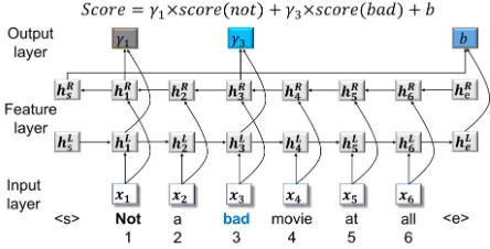
We investigate a method that can potentially ad-dress the above issues, by using a recurrent neu-ral network to capture context-dependent seman-tic composition effects over sentences. Shown in Figure 2, the model is conceptually simple, us-ing a weighted sum of lexicon sentiments and a sentence-level bias to estimate the sentiment value of a sentence. The key idea is to use a bi-directional long-short-term-memory (LSTM) (Hochreiter and Schmidhuber, 1997; Graves et al., 2013) model to capture global syntactic dependencies and seman-tic information, based on which the weight of each sentiment word together with a sentence-level sen-timent bias score are predicted. Such weights are context-sensitive, and can express flipping negation by having negative values.

The advantages of the recurrent network model over existing semantic-composition-aware discrete models such as (Choi and Cardie, 2008) include its capability of representing non-local and subtle se-mantic features without suffering from the challenge of designing sparse manual features. On the other hand, compared with neural network models, which recently give the state-of-the-art accuracies (Li et al., 2015; Tai et al., 2015), our model has the ad-vantage of leveraging sentiment lexicons as a useful resource. To our knowledge, we are the first to in-tegrate the operation into sentiment lexicons and a deep neural model for sentiment analysis.

The conceptually simple model gives strong em-pirical performances. Results on standard sentiment benchmarks show that our method gives competitive

Figure 2:Overall model structure. The sentiment score of the sentence “not a bad movie at all” is a weighted sum of the scores of sentiment words “not”, ”bad” and a sentence-level bias score b. score(not)andscore(bad)are prior scores obtained from sentiment lexicons.γ1andγ3are context-sensitive weights for

sentiment words “not” and “bad”, respectively.

accuracies to the state-of-the-art models in the liter-ature. As a by-product, the model can also correctly identify the compositional changes on the sentiment values of each word given a sentential context.

Our code is released at

https://github.com/zeeeyang/lexicon rnn.

2 Related Work

There exist many statistical methods that exploit sentiment lexicons (Kim and Hovy, 2004; Agarwal et al., 2011; Mohammad et al., 2013; Guerini et al., 2013; Tang et al., 2014b; Vo and Zhang, 2015; Cam-bria, 2016). Mohammad et al. (2013) leverage a large sentiment lexicon in a SVM model, achiev-ing the best results in the SemEval 2013 bench-mark on sentence-level sentiment analysis (Nakov et al., 2013). Compared to these methods, our model has two main advantages. First, we use a recurrent neural network to model context, thereby exploiting

non-localsemantic information. Second, our model offers context-sensitive operational details on each word.

Differ-ent from theserule-basedmethods, Choi and Cardie (2008) use a structured linear model tolearn seman-tic compositionality relying on a set ofmanual fea-tures. In contrast, we leverage a recurrent neural model for inducing semantic composition features

automatically. Our weighted-sum representation of semantic compositionality is formally simpler com-pared with fine-grained rules such as (Taboada et al., 2011). However, it is sufficient for describing the

resulting effect of complex and context-dependent operations, with the semantic composition process being modeled by LSTM. Our sentiment analyzer also enjoys a more competitive LSTM baseline com-pared to a traditional discrete models.

Our work is also related to recent work on us-ing deep neural networks for sentence-level senti-ment analysis, which exploits convolutional (Kalch-brenner et al., 2014; Kim, 2014; Ren et al., 2016), recursive (Socher et al., 2013; Dong et al., 2014; Nguyen and Shirai, 2015) and recurrent neural net-works (Liu et al., 2015; Wang et al., 2015; Zhang et al., 2016), giving highly competitive accuracies. As our baseline, LSTM (Tai et al., 2015; Li et al., 2015) stands among the best neural methods. Our model is different from these prior methods in mainly two aspects. First, we introduce sentiment lexicon fea-tures, which effectively improve classification ac-curacies. Second, we learn extra operation details, namely the weights on each word, automatically as hidden variables. While the baseline uses LSTM features to perform end-to-end mapping between sentences andsentiments, our model uses them to in-duce thelexicon weights, via which word level sen-timent are composed to derive sentence level senti-ment.

3 Model

Formally, given a sentence s = w1w2...wn and a

sentiment lexiconD, denote the subjective words in

s asw_jD₁w_jD₂...wD_jm. Our model calculates the

senti-ment score ofsaccording toDin the form of

Score(s) = m

X

t=1

γjtscore(w

D

jt) +b, (1)

whereScore(wD_jt)is the sentiment value ofwjt,γjt

are sentiment weights andbis a sentence-level bias.

The sentiment values of words and sentences are real

numbers, with the sign indicating the polarity and the absolute value indicating the strength.

As shown in Figure 2, our neural model consists of three main layers, namely the input layer, the

feature layerand theoutput layer. The input layer maps each word in the input sentence into a dense real-value vector. The feature layer exploits a bi-directional LSTM (Graves and Schmidhuber, 2005; Graves et al., 2013) to extract non-local semantic in-formation over the sequence. The output layer cal-culates a weight score for each sentiment word, as well as an overall sentiment bias of the sentence.

In this figure, the score of the sentence “not a bad movie at all” is decided by a weighted sum of the sentiments of “bad” and “not”1_{, and a sentiment}

shift bias based on the sentence structure. Ideally, the weight on “not” should be a small negative value, which results in a slightly positive sentiment shift. The weight on “bad” should be negative, which rep-resents a flip in the polarity. These weights jointly model a negation effect that involves both shifting and flipping.

3.1 Bidirectional LSTM

We use LSTM (Hochreiter and Schmidhuber, 1997) for feature extraction, which recurrently processes sentence stoken by token. For each word wt, the

model calculate a hidden state vectorht. A LSTM cell block makes use of an input gateit, a memory cellct, a forget gateftand an output gateotto con-trol information flow from the history x1...xt and h1...ht−1 to the current state ht. Formally, ht is computed as follows:

it=σ(Wixt+Uiht−1+Vict−1+bi) ft=1.0−it

gt= tanh(Wgxt+Ught₋1+bg) ct=ftct−1+itgt

ot=σ(Woxt+Uoht−1+Voct+bo) ht=ottanh(ct)

Herext is the word embedding of word wt, σ

de-notes the sigmoid function,is element-wise mul-tiplication.Wi,Ui,Vi,bi,Wg,Ug,bg,Wo,Uo, Voandbo are LSTM parameters.

We apply a bidirectional extension of LSTM (BiLSTM) (Graves and Schmidhuber, 2005; Graves et al., 2013), shown in Figure 2, to encode the input sentence s both left-to-right and right-to-left. The

BiLSTM model maps each word wt to a pair of

hidden vectors hL_t andhR_t, which denote the hid-den vector of the left-to-right LSTM and right-to-left LSTM, respectively. We use different parame-ters for the left-to-right LSTM and the right-to-left LSTM. These state vectors are used as features for calculating the sentiment weightsγ.

In addition, we append a sentence end marker

w<e>to the left-to-right LSTM and a sentence start

markerw<s>to the right-to-left LSTM. The hidden

state vector ofw<s> andw<e>are denoted as hRs andhL_e, respectively.

3.2 Output Layer

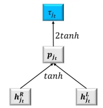
The base score. Given a lexicon word wjt in the sentences(wjt ∈D), we use the hidden state vec-tors hL_jt andhR_jt in the feature layer to calculate a weight valueτjt. As shown in Figure 3, a two-layer

neural network is used to induceτjt. In particular, a hidden layer combines hL_t and hR_t using a non-lineartanh activation

ps_jt = tanh(WL_pshL_jt+WR_pshR_jt+bps) (2)

The resulting hidden vectorps

jt is then mapped into τjt using anothertanhlayer.

τ_js_t = 2 tanh(Wpwpsjt+bpw) (3)

We choose the2tanhfunction to make the learned

weights conceptually useful. The factor 2 is in-troduced for modelling the effect of intensification. Since the range oftanhfunction is[−1,1], the range

of 2tanh is[₋2,2]. Intuitively, a weight value of

1 maps the word sentiment directly to the sentence sentiment, such as the weight for “good” in “This is good”. A weight value in(1,2]represents

intensifi-cation, such as the weight for “bad” in “very bad”. Similarly, a weight value in(0,1)represents

weak-ening, and a weight in (₋2,0) represents various

scales of negations.

Given all lexicon words wD_jt in the sentence, we

calculate a base score for the sentence

Sbase=

Pm

t=1τjtscore(wjDt)

m (4)

Figure 3:Weight score calculation.

By averaging the score of each word, the resulting

Sbaseis confined to[−2α,2α], whereαis the

maxi-mum absolute value of word sentiment. In the above equations, WL_ps, WR_ps, bps, Wpw and bpw are model parameters.

The bias score. We use the same neural network structure in Figure 3 to calculate the overall bias of the input sentence. The input to the neural network includeshR

s andhLe, and the output is a bias score

Sbias. Intuitively, the calculation of Sbias relies on

information of the full sentence. hR_s and hL_e are chosen because they have commonly been used in the research literature to represent overall sentential information (Graves et al., 2013; Cho et al., 2014).

We use a dedicated set of parameters for calculat-ing the bias, where

pB = tanh(WL_pbhL_e +WR_pbhR_s +bpb) (5)

and

Sbias= 2 tanh(WbpB+bp) (6) WL

pb, WRpb, bpb, WbandbLp are parameters.

3.3 Final Score Calculation

The base Sbase and bias Sbias are linearly

interpo-lated to derive the final sentiment value for the sen-tences.

Score(s) =λSbase+ (1−λ)Sbias (7)

λ_∈[0,1]reflects the relative importance of the base

score in the sentence. It offers a new degree of model flexibility, and should be calculated for each sen-tence specifically. We use the attention model (Bah-danau et al., 2014) to this end. In particular, the base score features hL_t/hR_t and the bias score fea-tureshL_e/hR_s are combined in the calculation

where

hbias =hLe ⊕hRs (9) and

hbase= Pm

t=1hLjt⊕h R jt

m (10)

Hereσdenotes the sigmoid activation function and

⊕ denotes vector concatenation. Wsλ, Wbλ and

bλ are model parameters.

The final score of the sentence is

Score(s) =λSbase+ (1−λ)Sbias

= λ m

m

X

t=1

τjtscore(w

D

jt) + (1−λ)Sbias

This corresponds to the original Equation 1 byγjt =

λ

mτjt andb= (1−λ)Sbias. 3.4 Training and Testing

Our training data contains two different settings. The first is binary sentiment classification. In this task, every sentencesiis annotated with a sentiment

labelli, whereli= 0andli = 1to indicate negative

and positive sentiment, respectively. We apply logis-tic regression on the output layer. Denote the proba-bility of a sentencesibeing positive and negative as p1

si andp

0

si respectively.p

0 si andp

1

si are estimated as

p1_si =σ(Score(si))

p0_si = 1₋p1_si (11)

Suppose that there areN training sentences, the loss

function over the training set is defined as

L(Θ) =−

N

X

i=1

logpli

si+

λr 2 ||Θ||

2_{, (12)}

whereΘis the set of model parameters. λris a

pa-rameter for L2 regularization.

The second setting is multi-class classification. In this task, every sentencesi is assigned a sentiment

labelli from 0 to 4, which representvery negative, negative,neutral,positiveandvery positive, respec-tively. We apply least square regression on the out-put layer. Since the outout-put range of2tanhis [-2, 2],

the value of the base score and the bias score both belongs to [-2, 2]. The final score is a weighted sum of the base score and the bias score, also belonging to [-2, 2]. However, the gold sentiment label ranges

Positive Negative Total

Train 3,009 1,187 4,196

Dev 483 283 766

Test 1,313 490 1,803

Table 1:Statistics of the Twitter dataset.

Task Label _SentencesTraining _SentencesDev _SentencesTest

5-class

-2 1,092 139 279

-1 2,218 289 633

0 1,624 229 389

1 2,322 279 510

2 1,288 165 399

2-class 0₁ 3,310_3,610 444₄₂₈ 909₉₁₂

Table 2:Statistics of SST.

from 0 to 4. We add an offset -2 to every gold sen-timent label to both adapt our model to the train-ing data and to increase the interpretability of the learned weights. The loss function for this problem is then defined as

L(Θ) = N

X

i=1

(Score(si)−li)2+ λr

2 ||Θ||

2 ₍₁₃₎

During testing, we predict the sentiment labell∗_i of

a sentencesiby

l_i∗=

              

−2 if Score(si)≤ −1.5

−1 if −1.5< Score(si)≤ −0.5 0 if −0.5< Score(si)≤0.5 1 if 0.5< Score(si)≤1.5 2 if Score(si)>1.5

(14)

4 Experiments

4.1 Experimental Settings

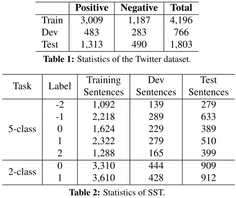
Data. We test our model on three datasets, includ-ing a dataset on Twitter sentiment classification, a dataset on movie review and a dataset with mixed domains. The Twitter dataset is taken from Se-mEval 2013 (Nakov et al., 2013). We downloaded the dataset according to the releasedids. The statis-tics of the dataset are shown in Table 1.

The movie review dataset is Stanford Sentiment Treebank2_{(SST) (Socher et al., 2013). For each}

Polarity books dvds electronics music videogames

Positive 19 19 19 20 20

Negative 29 20 19 20 20

Table 3:Document distribution of the mixed domain dataset.

tree is given. Each internal constituent node is an-notated with a sentiment label ranging from 0 to 4. We follow Socher et al. (2011) and Li et al. (2015) to perform five-class and binary classification, with the data statistics being shown in Table 2.

In order to examine cross-domain robustness, we apply our model on a product review cor-pus (T¨ackstr¨om and McDonald, 2011), which con-tains 196 documents covering 5 domains: books, dvds, electronics, music and videogames. The doc-ument distribution is listed in Table 3.

Lexicons. We use four sentiment lexicons, namely TS-Lex, S140-Lex, SD-Lex and SWN-Lex. TS-Lex3 _{is a large-scale sentiment lexicon built}

from Twitter by Tang et al. (2014a) for learning sentiment-specific phrase embeddings. S140-Lex4

is the Sentiment140 lexicon, which is built from point-wise mutual information using distant super-vision (Go et al., 2009; Mohammad et al., 2013).

SD-Lex is built from SST. We construct a sen-timent lexicon from the training set by excluding all neutral words and adding the aforementioned offset -2 to each entry. SWN-Lex is a sentiment lexicon extracted from SentimentWordNet3.0 (Bac-cianella et al., 2010). For words with different part-of-speech tags, we keep the minimum negative score or the maximum positive score. The original score in the SentimentWordNet3.0 is a probability value between 0 and 1, and we scale it to [-2, 2]5_.

When building these lexicons, we only use the sentiment scores for unigrams. Ambiguous words are discarded. Both TS-Lex and S140-Lex are Twitter-specific sentiment lexicons. They are used in the Twitter sentiment classification task. SD-Lex and SWN-Lex are exploited for the Stanford dataset. The statistics of lexicons are listed in Table 4.

3_{http://ir.hit.edu.cn/ dytang/paper/14coling/data.zip} 4 http://saifmohammad.com/Lexicons/Sentiment140-Lexicon-v0.1.zip

5_{Taboada et al. (2011) also mentioned two methods to derive} sentiment score for a sentiment word from SentimentWordNet. We leave them for future work.

Lexicon Positive Negative Total

SD-Lex 2,547 2,448 4,995 SWN-Lex 15,568 17,412 32,980 TS-Lex 33,997 32,026 66,023 S140-Lex 24,156 38,312 62,468

Table 4:Statistics of sentiment lexicons.

4.2 Implementation Details

We implement our model based on the CNN toolkit.6 _{Parameters are optimized using stochastic}

gradient descent with momentum (Sutskever et al., 2013). The decay rate is 0.1. For initial learning rate, L2 and other hyper-parameters, we adopt the default values provided by the CNN toolkits. We select the best model parameter according to the classification accuracy on the development set.

For the Twitter data, we use theglove.twitter.27B7

as pretrained word embeddings. For the Stan-ford dataset, following Li et al. (2015), we use

glove.840B.300d8 _{as pretrained word embeddings.}

Words that do not exist in both the training set and the pretrained lookup table are treated as out-of-vocabulary (OOV) words. Following Dyer et al. (2015), singletons in the training data are ran-domly mapped to UNK with a probabilitypunk

dur-ing traindur-ing. We set punk = 0.1. All word

em-beddings are fine-tuned. We use dropout (Srivastava et al., 2014) in the input layer to prevent overfitting during training.

One-layered BiLSTM is used for all tasks. The dimension of the hidden vector in LSTM is 150. The size of the second layer in Figure 3 is 64.

4.3 Development Results

Table 5 shows results on the Twitter development set. Bi-LSTM is our model using the bias score

Sbias only, which is equivalent to bidirectional

LSTM model of Li et al. (2015) and Tai et al. (2015), since they use same features and only dif-fer in the output layer. Bi-LSTM+avg.lexicon is a baseline model integrating the average sen-timent scores of lexicon words as a feature, and Bi-LSTM+flex.lexicon is our final model, which considers both the Bi-LSTM score (Sbias) and the

context-sensitive score (Sbase). 6_{https://github.com/clab/cnn}

Method Dict Dev(%)

Bi-LSTM None 84.2

Bi-LSTM+avg.lexicon S140-Lex 84.9 Bi-LSTM+flex.lexicon S140-Lex 86.4

Table 5:Results on the Twitter development set.

Method Test(%)

SVM6 (Zhu et al., 2014) 78.5 Tang et al. (2014a) 82.4

Bi-LSTM 86.7

Bi-LSTM + TS-Lex 87.6 Bi-LSTM + S140-Lex 88.0

Table 6:Results on the Twitter test set.

Bi-LSTM+avg.lexicon improves the classifica-tion accuracy over Bi-LSTM by 0.7 point, which shows the usefulness of sentiment lexicons to re-current neural models using a vanilla method. It is consistent with previous research on discrete

models. By considering context-sensitive weight-ing for sentiment wordsBi-LSTM+flex.lexicon fur-ther outperforms Bi-LSTM+avg.lexicon, improv-ing the accuracy by 1.5 points (84.9→86.4), which

demonstrates the strength of context-sensitive scor-ing. Base on the development results, we use Bi-LSTM+flex.lexiconfor the remaining experiments. 4.4 Main Results

Twitter.Table 6 shows results on the Twitter test set. SVM6is our implementation of Zhu et al. (2014), which extracts six types of manual features from TS-Lex for SVM classification. The features include: (1) the number of sentiment words in the sentence; (2) the total sentiment scores of the sentence; (3) the maximum sentiment score; (4) the total positive and negative sentiment scores; (5) the sentiment score of the last word in the sentence. The system of Tang et al. (2014a) is a state-of-the-art system that ex-tracts various manually designed features from TS-Lex, such as bag-of-words, term frequency, parts-of-speech, the sum of sentiment scores of all words in a tweet, etc, for SVM. TheBi-LSTMrows are our final models with different lexicons.

Both SVM6and Tang et al. (2014a) exploit dis-crete features. Compared to them,Bi-LSTMgives better accuracies without using lexicons, which demonstrates the relative strength of deep neural net-work for sentiment analysis. Compared with Tang et al. (2014a), ourBi-LSTM+TS-Lexmodel improves

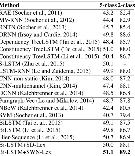
Method 5-class 2-class

RAE (Socher et al., 2011) 43.2 82.4 MV-RNN (Socher et al., 2012) 44.4 82.9 RNTN (Socher et al., 2013) 45.7 85.4 DRNN (Irsoy and Cardie, 2014) 49.8 88.6 Dependency TreeLSTM (Tai et al., 2015) 48.4 85.7 Constituency TreeLSTM (Tai et al., 2015) 51.0 88.0 Constituency TreeLSTM (Li et al., 2015) 50.4 86.7 S-LSTM (Zhu et al., 2015) 50.1 -LSTM-RNN (Le and Zuidema, 2015) 49.9 88.0 CNN-non-static (Kim, 2014) 48.0 87.2 CNN-multichannel (Kim, 2014) 47.4 88.1 DCNN (Kalchbrenner et al., 2014) 48.5 86.8 Paragraph-Vec (Le and Mikolov, 2014) 48.7 87.8 NBoW (Kalchbrenner et al., 2014) 42.4 80.5 SVM (Socher et al., 2013) 40.7 79.4 BiLSTM (Tai et al., 2015) 49.1 87.5 BiLSTM (Li et al., 2015) 49.8 86.7 Hier-Sequence (Li et al., 2015) 50.7 86.9

Bi-LSTM+SD-Lex 50.0 88.1

Bi-LSTM+SWN-Lex 51.1 89.2

Table 7:Results on SST.5-classshows fine-grained classifica-tion. The last block lists our results.

the sentiment classification accuracy from 82.4 to 87.6, which again shows the strength of

context-sensitive features. S140-Lex gives slight improve-ments over TS-Lex.

SST. Table 7 shows the results on SST. We in-clude various results of recursive (the first block), convolutional (the second block), and sequential LSTM models (the fourth block). These neural mod-els give the recent state-of-the-art on this dataset. Our method achieves highly competitive accuracies. In particular, compared to sequential LSTMs, our best model gives the top result both on the binary and fine-grained classification task. This shows the usefulness of lexicons to neural models. In addition, SWN-Lex gives better results compared with SD-Lex. This is intuitive because SD-Lex is a smaller lexicon compared to SWN-Lex (4,999 entries v.s. 32,980 entries). SD-Lex does not bring external knowledge to this dataset, while SWN-Lex does.

Model Train Test Books Dvds Electronics Music Videogames Average

Bi-LSTM None None 71.79 89.74 65.79 95 85 81.63

Bi-LSTM+flex.lexicon SD-Lex SD-Lex 76.92 84.62 78.95 92.5 80 82.65 Bi-LSTM+flex.lexicon SD-Lex SWN-Lex 82.05 92.31 73.68 92.5 80 84.18 Bi-LSTM+flex.lexicon SWN-Lex SWN-Lex 84.62 92.31 68.42 100 85 86.22

Table 8:Cross-domain sentiment analysis. Training domain is movie review.

Figure 4:Sentiment composition examples.

of sentences to the document level. We compare the effects of different lexicons over a baseline Bi-LSTM trained on SST (movie domain).

Table 8 shows the results. Introducing the sen-timent lexicons SD-Lex and SWN-Lex consistently improves the classification accuracy across five do-mains compared with the baselineBi-LSTMmodel. When trained and tested using the same lexicon, SWN-Lex gives better performances on three out of five domains. SD-Lex gives better results only on Electronics. This shows that the results are sensi-tive to the domain of the sentiment lexicon, which is intuitive.

We also investigate a model trained using SD-Lex but tested by replacing SD-SD-Lex with SWN-SD-Lex. This is to examine the generalizability of a source-domain model on different target source-domains by plug-ging in relevant domain-specific lexicons, without being retrained. Results show that the mode still out-performs the SD-Lex lexicon on two out of five do-mains, but is less accurate than full retraining using SWN-Lex.

4.5 Discussion

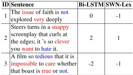
Figure 4 shows the details of sentiment composition for two sentences in the SST, learned automatically by our model. For the first sentence, the three sub-jective words in the lexicon “pure”, “excitement”

ID Sentence Bi-LSTM SWN-Lex

1 The_exploredissue_veryof faith is_deeplynot 0 -1

2

Steers turns in asnappy screenplay that curls at the edges; it ’s soclever youwanttohateit.

2 1

3 A film soimpossibletedioustocarethat it iswhether

that boast istrueornot. -2 -1

Table 9:Example predictions made by the Bi-LSTM model and our Bi-LSTM+SWN-Lex model for fine-grained classification task.Redwords andbluewords are positive and negative entries in the SentimentWordNet3.0 lexicon, respectively.

and “not” receives weights of 1.6, 1.9 and −0.6,

respectively, and the overall bias of the sentence is positive. A λ value (0.58) that slightly biases

to-wards the base score leads to a final sentiment score is1.8, which is close to the gold label 2.

In the second example, both negation words re-ceived positive weight values, and the bias over the sentence is negative. A λ (0.3) value that biases

towards the bias score results in a final score of

−1.2, which is close to the gold label −1. These

results demonstrate the capacity of the model to de-cide how word-level sentiments composite accord-ing to sentence-level context.

Table 9 shows three sentences in the Stanford test set which are incorrectly classified by LSTM model, but correctly labeled by our Bi-LSTM+SWN-Lex model. These examples show that our model is more sensitive to context-dependent sentiment changes, thanks to the use of lexicons as a basis.

5 Conclusion

averag-ing method in traditional bag-of-word models, our system leverages the strength of semantic feature learning by LSTM models to calculate a context-dependent weight for each word given an input sen-tence. The method gives competitive results on var-ious sentiment analysis benchmarks. In addition, thanks to the use of lexicons, our model can im-prove the cross-domain robustness of recurrent neu-ral models for sentiment analysis.

Acknowledgments

Yue Zhang is the corresponding author. Thanks to anonymous reviewers for their helpful com-ments and suggestions. Yue Zhang is supported by NSFC61572245 and T2MOE201301 from Sin-gapore Ministry of Education.

References

Apoorv Agarwal, Boyi Xie, Ilia Vovsha, Owen Rambow, and Rebecca Passonneau. 2011. Sentiment analysis of twitter data. In Proceedings of the Workshop on Languages in Social Media, pages 30–38.

Stefano Baccianella, Andrea Esuli, and Fabrizio Sebas-tiani. 2010. Sentiwordnet 3.0: An enhanced lexical resource for sentiment analysis and opinion mining. In Proceedings of LREC, volume 10, pages 2200–2204. Dzmitry Bahdanau, Kyunghyun Cho, and Yoshua

Ben-gio. 2014. Neural machine translation by jointly learning to align and translate. CoRR, abs/1409.0473. Erik Cambria. 2016. Affective computing and sentiment

analysis. IEEE Intelligent Systems, 31(2):102–107. Kyunghyun Cho, Bart van Merrienboer, Caglar Gulcehre,

Dzmitry Bahdanau, Fethi Bougares, Holger Schwenk, and Yoshua Bengio. 2014. Learning phrase represen-tations using rnn encoder–decoder for statistical ma-chine translation. In Proceedings of EMNLP, pages 1724–1734.

Yejin Choi and Claire Cardie. 2008. Learning with com-positional semantics as structural inference for subsen-tential sentiment analysis. InProceedings of EMNLP, pages 793–801.

Kerstin Denecke. 2009. Are sentiwordnet scores suited for multi-domain sentiment classification? InICDIM, pages 1–6. IEEE.

Ann Devitt and Khurshid Ahmad. 2007. Sentiment polarity identification in financial news: A cohesion-based approach.

Xiaowen Ding, Bing Liu, and Philip S Yu. 2008. A holis-tic lexicon-based approach to opinion mining. In

Pro-ceedings of the 2008 International Conference on Web Search and Data Mining, pages 231–240.

Li Dong, Furu Wei, Chuanqi Tan, Duyu Tang, Ming Zhou, and Ke Xu. 2014. Adaptive recursive neural network for target-dependent twitter sentiment classi-fication. InProceedings of ACL, pages 49–54. Chris Dyer, Miguel Ballesteros, Wang Ling, Austin

Matthews, and Noah A. Smith. 2015. Transition-based dependency parsing with stack long short-term memory. InACL.

Andrea Esuli and Fabrizio Sebastiani. 2006. Sentiword-net: A publicly available lexical resource for opinion mining. In Proceedings of LREC, volume 6, pages 417–422.

Alec Go, Richa Bhayani, and Lei Huang. 2009. Twit-ter sentiment classification using distant supervision. CS224N Project Report, Stanford, 1:12.

Alex Graves and J¨urgen Schmidhuber. 2005. Frame-wise phoneme classification with bidirectional lstm and other neural network architectures. Neural Net-works, 18(5):602–610.

A. Graves, A. Mohamed, and G. Hinton. 2013. Speech recognition with deep recurrent neural networks. Marco Guerini, Lorenzo Gatti, and Marco Turchi. 2013.

Sentiment analysis: How to derive prior polarities from SentiWordNet. InProceedings of EMNLP, pages 1259–1269.

Sepp Hochreiter and J¨urgen Schmidhuber. 1997. Long short-term memory. Neural computation, 9(8):1735– 1780.

Minqing Hu and Bing Liu. 2004. Mining and summariz-ing customer reviews. InProceedings of KDD, KDD ’04, pages 168–177.

Ozan Irsoy and Claire Cardie. 2014. Deep recursive neural networks for compositionality in language. In Advances in Neural Information Processing Systems, pages 2096–2104.

Nal Kalchbrenner, Edward Grefenstette, and Phil Blun-som. 2014. A convolutional neural network for mod-elling sentences. InProceedings of ACL, pages 655– 665.

Colm Kearney and Sha Liu. 2014. Textual sentiment in finance: A survey of methods and models. Interna-tional Review of Financial Analysis, 33:171–185. Soo-Min Kim and Eduard Hovy. 2004. Determining the

sentiment of opinions. InProceedings of the 20th in-ternational conference on Computational Linguistics, page 1367.

Yoon Kim. 2014. Convolutional neural networks for sen-tence classification. InProceedings of EMNLP, pages 1746–1751.

Quoc V. Le and Tomas Mikolov. 2014. Distributed representations of sentences and documents. CoRR, abs/1405.4053.

Phong Le and Willem Zuidema. 2015. Compositional distributional semantics with long short term memory. InProceedings of the Fourth Joint Conference on Lex-ical and Computational Semantics, pages 10–19. Jiwei Li, Minh-Thang Luong, Dan Jurafsky, and Eudard

Hovy. 2015. When are tree structures necessary for deep learning of representations?

Pengfei Liu, Xipeng Qiu, Xinchi Chen, Shiyu Wu, and Xuanjing Huang. 2015. Multi-timescale long short-term memory neural network for modelling sentences and documents. In Proceedings of EMNLP, pages 2326–2335.

Saif M. Mohammad, Svetlana Kiritchenko, and Xiaodan Zhu. 2013. Nrc-canada: Building the state-of-the-art in sentiment analysis of tweets. InProceedings of SemEval-2013, June.

Karo Moilanen and Stephen Pulman. 2007. Sentiment composition.

Richard Montague. 1974. Formal Philosophy: Selected Papers of Richard Montague. Ed. and with an Introd. by Richmond H. Thomason. Yale University Press. Preslav Nakov, Sara Rosenthal, Zornitsa Kozareva,

Veselin Stoyanov, Alan Ritter, and Theresa Wilson. 2013. Semeval-2013 task 2: Sentiment analysis in twitter. In Second Joint Conference on Lexical and Computational Semantics (*SEM), Volume 2: Pro-ceedings of SemEval-2013, pages 312–320.

Thien Hai Nguyen and Kiyoaki Shirai. 2015. Phrasernn: Phrase recursive neural network for aspect-based sen-timent analysis. InProceedings of EMNLP.

Livia Polanyi and Annie Zaenen. 2006. Contextual va-lence shifters. InComputing attitude and affect in text: Theory and applications, pages 1–10.

Yafeng Ren, Yue Zhang, Meishan Zhang, and Donghong Ji. 2016. Context-sensitive twitter sentiment classifi-cation using neural network. InProceedings of AAAI. Richard Socher, Jeffrey Pennington, Eric H. Huang,

An-drew Y. Ng, and Christopher D. Manning. 2011. Semi-Supervised Recursive Autoencoders for Pre-dicting Sentiment Distributions. In Proceedings of EMNLP.

Richard Socher, Brody Huval, Christopher D. Manning, and Andrew Y. Ng. 2012. Semantic compositionality through recursive matrix-vector spaces. In Proceed-ings of EMNLP, pages 1201–1211.

Richard Socher, Alex Perelygin, Jean Wu, Jason Chuang, D. Christopher Manning, Andrew Ng, and Christopher Potts. 2013. Recursive deep models for semantic compositionality over a sentiment treebank. In Pro-ceedings of EMNLP, pages 1631–1642.

Nitish Srivastava, Geoffrey Hinton, Alex Krizhevsky, Ilya Sutskever, and Ruslan Salakhutdinov. 2014. Dropout: A simple way to prevent neural networks from overfitting. The Journal of Machine Learning Research, 15(1):1929–1958.

Ilya Sutskever, James Martens, George Dahl, and Geof-frey Hinton. 2013. On the importance of initialization and momentum in deep learning. In Proceedings of the 30th international conference on machine learning (ICML-13), pages 1139–1147.

Maite Taboada, Julian Brooke, Milan Tofiloski, Kimberly Voll, and Manfred Stede. 2011. Lexicon-based meth-ods for sentiment analysis.Computational linguistics, 37(2):267–307.

Oscar T¨ackstr¨om and Ryan McDonald. 2011. Discov-ering fine-grained sentiment with latent variable struc-tured prediction models. InAdvances in Information Retrieval, pages 368–374.

Kai Sheng Tai, Richard Socher, and Christopher D. Man-ning. 2015. Improved semantic representations from tree-structured long short-term memory networks. In Proceedings of ACL, pages 1556–1566.

Duyu Tang, Furu Wei, Bing Qin, Ming Zhou, and Ting Liu. 2014a. Building large-scale twitter-specific sen-timent lexicon : A representation learning approach. InProceedings of COLING, pages 172–182, August. Duyu Tang, Furu Wei, Nan Yang, Ming Zhou, Ting Liu,

and Bing Qin. 2014b. Learning sentiment-specific word embedding for twitter sentiment classification. InProceedings of ACL, pages 1555–1565, June. Peter Turney. 2002. Thumbs up or thumbs down?

se-mantic orientation applied to unsupervised classifica-tion of reviews. InProceedings of ACL.

Duy-Tin Vo and Yue Zhang. 2015. Target-dependent twitter sentiment classification with rich automatic features. InProceedings of IJCAI, pages 1347–1353, July.

Xin Wang, Yuanchao Liu, Chengjie SUN, Baoxun Wang, and Xiaolong Wang. 2015. Predicting polarities of tweets by composing word embeddings with long short-term memory. In Proceedings of ACL, pages 1343–1353.

Theresa Wilson, Janyce Wiebe, and Paul Hoffmann. 2005. Recognizing contextual polarity in phrase-level sentiment analysis. InProceedings of HLT-EMNLP. Meishan Zhang, Yue Zhang, and Duy-Tin Vo. 2016.

Gated neural networks for targeted sentiment analysis. Xiaodan Zhu, Svetlana Kiritchenko, and Saif M Moham-mad. 2014. Nrc-canada-2014: Recent improvements in the sentiment analysis of tweets.