Abstract— Preventive maintenance (PM) can benefit systems
having an increasing failure rate. However, PM is often scheduled in order to minimize the maintenance cost or to comply with production planning requirements or instruction from the equipment suppliers. Given that maintenance actions affect process time variability and resource utilization, such maintenance planning criteria may cause other adverse effects on the operational performance of the manufacturing system such as an increase in Work In Process (WIP) and cycle time. In this paper some approximate queueing models are utilize to asses the impact of PM interval on WIP. It is shown that WIP value is strongly influenced by the PM interval and that maintenance intervals corresponding to a minimum maintenance cost or minimum WIP can be quite different. This kind of analysis can help in making more informed decisions involving WIP and cost trade-offs.
Index Terms— Maintenance optimization, manufacturing
systems performances, preventive maintenance, queueing models.
I. INTRODUCTION
Manufacturing systems are subject to deterioration with usage and age. In case of repairable systems, maintenance can restore the operational status of manufacturing equipment after failures or can preserve it by reducing the occurrence of breakdowns. However, maintenance downtimes increase resources utilization and system variability, negatively affecting some relevant performance measures of manufacturing systems, such as work in process (WIP) and cycle time. While a vast body of literature about maintenance planning and optimization exists [1]-[5], the interactions between maintenance planning and manufacturing systems performances has been scarcely investigated. In particular, some criteria have been proposed to dynamically determine maintenance actions based on the system status [6]-[7] and to control manufacturing systems taking into account machines breakdowns [8]-[9]. However, most of these approaches are quite complex and difficult to apply in real life conditions. In this paper, instead, some easy to use approximate queueing models are utilized to assess the impact that preventive maintenance interval has on manufacturing systems performance, mainly focusing on WIP. This is made to show how the arbitrary selection of preventive maintenance interval or maintenance scheduling
Manuscript received April 16, 2009.
A. C. Caputo is with the University of L’Aquila, L’Aquila, Italy (phone: +39-0862-434312; fax: +39-0862-434303; e-mail:
P. Salini is with the University of L’Aquila, L’Aquila, Italy (e-mail: [email protected]).
based on minimum maintenance cost approaches can be detrimental to WIP and cycle time, so that trade-off decision may be required.
The paper is organized as follows. At first a brief review of preventive maintenance optimization approaches based on cost minimization is carried out. Then, available queueing models for unreliable servers are surveyed to select suitable analytical tools to estimate the performance of manufacturing systems subject to corrective and preventive maintenance. Subsequently, the chosen queueing models are utilized in a comparative manner to explore the behaviour of a single machine system. Some analytical results are presented and discussed in order to point out the relevant issues to maintenance planners. This allows more informed decisions.
II. ECONOMIC OPTIMIZATION OF PREVENTIVE MAINTENANCE SCHEDULE
In systems having an increasing failure rate (IFR), preventive maintenance bringing the system into its original state (as good as new) is beneficial as it reduces the average failure rate. The problem then arises of determining the preventive maintenance interval TP. This is usually selected by maintenance planners in order to respect some external requirement (such as instructions from the equipment manufacturers or directives from the production planning department) or, too often, is decided arbitrarily. In case one wishes to optimize TP, a maintenance cost minimization approach is usually pursued. In this respect many policies exist [1]-[5] which mostly fall into two classes, namely age replacement policies and periodic replacement policies. In age replacement policy a unit is always replaced at failure or time TP if it has not failed up to time TP. In both cases an “as good as new” intervention is assumed which means that the failure rate is restored to its initial value. In periodic replacement policy, instead, a unit is replaced periodically at planned times kTP(k = 1, 2, . . . ). Only minimal repair after each failure is made so that the failure rate remains undisturbed by any repair of failures between successive replacements performed at times kTP.
The preventive maintenance interval TP is often chosen to minimize the overall maintenance cost including both the cost of corrective repairs after a breakdown and planned preventive replacements. Over an infinite time horizon one usually refers to the expected maintenance cost per unit time of a maintenance cycle. In case of age replacement policy the average cost per unit time CAU (TP)
[
]
[
1 ( )]
) ( )
(
) ( 1 ) ( )
(
P P
P P
P B
P P P
AU
T R T MTTF T
R T
T R C T R C T
C
− +
− +
= (1)
Influence of Preventive Maintenance Policy on
Manufacturing Systems Performances
is computed as the ratio of the average maintenance cost over a cycle to the average cycle duration. In (1) CP is the cost of a preventive maintenance intervention and CB is the cost of a corrective intervention following a breakdown, R(TP) is the reliability computed over the preventive maintenance interval. MTTF is the average time to failure computed when a preventive maintenance with as good as new repair policy is adopted [10]
)
(
1
)
(
0P T
T
R
dt
t
R
MTTF
P
−
=
∫
(2)Assuming a Weibull distributed time to failure with parameters β an η, the reliability R(t) is [10]
β
η ⎟⎟⎠ ⎞ ⎜⎜ ⎝ ⎛ −
=
te
t
R
(
)
. (3)In case of periodic replacement, TP is the fixed cycle length and the average number of corrective repairs N(TP) expected over the cycle length is given by renewal theory
∫
=
TPB
P
t
dt
T
N
0
(
)
)
(
λ
(4)1
)
(
−
⎟⎟
⎠
⎞
⎜⎜
⎝
⎛
=
β
η
η
β
λ
Bt
t
(5)where λB(t) is the failure rate function [10]. Therefore, the maintenance cost per unit time is
P P B P P AU
T
T
N
C
C
T
C
(
)
=
+
(
)
. (6)Since with short TP one has high preventive maintenance costs but low corrective maintenance costs, while for long TP the opposite occurs, an optimal value of TP which minimizes CAU (TP) may exist and numerical methods can be used to determine it. However, this widely practiced approach only focuses on costs but neglects other performance measures of a manufacturing system which may be worsened by an unsuitable choice of TP. In fact, the preventive maintenance interval besides affecting the average failure rate and maintenance cost, also influences resource availability and utilization, as well as the variability of effective processing times, thus determining congestion problems which may increase WIP accumulation and cycle time at the workstations.
III. QUEUEING MODELS FOR UNRELIABLE MACHINES Queueing theory provides a convenient manner to quickly estimate the main performance measures of dynamic systems in which discrete events alter the state of the system. In queueing systems customers (i.e. jobs) arrive by some arrival
process and wait in queue for the next available server (i.e. a machine). When the server becomes available a customer is selected from the queue and serviced according to some discipline before leaving the system. Analytical queueing models provide generalizable results and explicitly show the role of the influencing parameters, while this is generally not possible in discrete events computer simulation models. The latter, on the other hand, are much more flexible and powerful, but are very time consuming to create and validate. Queueing theory [11] is often utilized to study manufacturing systems and a number of textbook are available on this subject [12]-[14]. However, even if from a long time a number of queueing models have been developed for unreliable servers [15]-[17], most of them are based on the assumption of exponentially distributed time to failure (i.e. constant failure rate) and only address preemptive interruptions, such as breakdowns, or non-preemptive such as preventive maintenance. This prevents from using simple queueing models to optimize maintenance policies as one need to model both kind of interruptions. Moreover the assumption of constant failure rate makes the models unsuitable to the case of preventive maintenance which is only useful when the system shows an increasing failure rate caused by progressive wear and deterioration. Furthermore, due to the complex nature of interruptions in manufacturing, it is often difficult to properly select the appropriate model. To this end Wu et al. [18] propose a useful classification. They at first distinguish between preemptive and non-preemptive interruptions. Preemptive interruptions are unscheduled and can occur during the processing of a job, thus inflating the average process time respect the value of the natural process time. Non-preemptive interruptions, instead, are usually scheduled and, in any case, can be postponed until the job processing is terminated. Then they distinguish between run-based and time-based interruptions. Run-based interruptions can occur only if WIP exist in the system or are indirectly caused by the presence of WIP. For instance the breakage of a tool can occur only if the machine is processing a part. Time-based interruptions instead can occur even in absence of WIP. Examples of run-based and time-based preemptive interruptions are, for instance, breakdowns or out of spec inputs, and power outages respectively. Cases of run-based and time-based non-preemptive interruptions instead are, for instance, setups and preventive maintenance respectively. Finally, they further consider state-induced or product-induced events as sub-cases of run-based non-preemptive events (i.e. a state-induced event is an interruption deriving from a change of state of the machine such as a warm up period when the machine passes from stand-by to working conditions). According to this classification, in this work we are interested in run-based preemptive events (i.e breakdowns) and time-based non-preemptive events (i.e. preventive maintenance.).
While the reader can consult the paper of Wu et al. [18] for a more complete classification of M/M/1, M/G/1 and G/G/1 queueing models referring to run-based or time-based interruptions when the uptime is exponentially distributed, here we consider only models for queues with Poisson arrivals and general service processes in single servers applications (M/G/1), which better fit the scope of this paper.
processes in single servers applications (G/G/1), the queueing time (QT) can be estimated as,
e e a
t
c
c
QT
E
⎟⎟
⎠
⎞
⎜⎜
⎝
⎛
−
⎟⎟
⎠
⎞
⎜⎜
⎝
⎛
+
=
ρ
ρ
1
2
)
(
2 2 (7)where ca is the coefficient of variation of interarrival time, ce is the coefficient of variation of effective process time, ρ= λ/μA is the resource utilization, A the breakdown induced server availability, te is the expected value of the Effective Process Time (EPT). EPT represents the average effective process time as modified respect the average natural process time t0 to account for the interruptions. Please note that this definition of te does not include state-induced, run-based non-preemptive events. In case of Poisson arrivals obviously
ca = 1. Hopp and Spearman [20] provide the following equations to compute the parameters of (7) in case of either preemptive or non-preemptive run-based events.
a a a t c σ
= (8)
Preemptive interruptions
A t te
0
= (9)
MTTR A t A MTTR A r e 0 2 2 2 2 0
2=
σ
+( +σ
)(1− )σ
(10)0 2 2
0
2 (1 ) (1 )
t MTTR A A c c c r e − + +
= (11)
Non-preemptive interruptions t t e
N
t
t
t
=
0+
(12)2 2 2 2 0 2 1 t t t t t e t N N N − + + =
σ
σ
σ
(13)2 2 2 e e e
t
c
=
σ
(14)In (8) to (14) ta is the average interarrival time and σa its standard deviation. σ0 is the standard deviation of natural process time, MTTR and σr the mean value and standard deviation of time to repair, c0 is the coefficient of variation of natural process time, cr is the coefficient of variation of repair time, tt is the average duration of non-preemptive interruption, σt its standard deviation, and Nt is the average number of jobs processed between non-preemptive interruptions.
In case one deals with both preemptive and non-preemptive interruptions Hopp and Spearman [20] suggest at first to compute the te and σevalues including only
preemptive interruptions through (9) - (10) and then to use such values as actual starting values t0σ0to compute the final
te and σevalues from (12)-(13).
Unfortunately, (11) is valid only in case of constant failure rate, and an explicit analytical expression for the coefficient of variation of effective process time with increasing failure rate is difficult to obtain. Moreover (13) could be used only to account for setups but not for preventive maintenance as the latter is useless in case of constant failure rate while when the failure rate is increasing the maintenance interval Nt influences the actual vale of the MTTF so that the above described two-step procedure can not be applied. Finally, Wu et al [18] point out that this model does not account for time-based and state-induced events.
A model such as the above one could be used as an approximation for cases including both preemptive and non-preemptive interruptions, provided that one includes in the effective process time the “inflation” effect of both breakdowns and preventive maintenance interruptions. However, the problem remains the estimation of ce in case of increasing failure rate and non-preemptive interruptions.
A model for M/G/1 non-preemptive priority queues with two priorities, by Adan and Resing [21], can be instead utilized as an approximation for time-based non preemptive interruptions cases, provided that average value of the process time is corrected to account for the effects of preemptive interruptions. According to this model λ1 and λ2 are the arrival rates of high and low priority jobs and μ1 and μ2 the service rates of high and low priority jobs respectively. Here the low priority jobs are the preventive maintenance interruptions.
This model computes the expected cycle time CT as
) ( ) ( ) ( ) ( 2 2 1 2 1 2 1
1 E S E S
QT E CT E λ λ λ λ λ λ + + + +
= (15)
) 1 ( ) 1 ( ) ( ) ( ) ( 1 ) ( ) ( ) ( ) ( ) ( ) ( 1 2 1 2 2 1 1 2 1 2 2 1 1 1 2 2 1 2 1 2 1 1 ρ ρ ρ ρ ρ ρ ρ ρ λ λ λ λ λ λ − − − + = − + = + + + = R E R E QT E R E R E QT E QT E QT E QT E (16)
S1 and S2 are the effective process times, ρ1= λ1/μ1, ρ2= λ2/μ2, while
2 , 1 ) ( 2 ) ( ) ( 2 = = i S E S E R E i i
i (17)
This model explicitly accounts for time-based non-preemptive interruptions (i.e. preventive maintenance) while preemptive interruptions should be included in the computation of effective process time S1.
IV. IMPACT OF PREVENTIVE MAINTENANCE INTERVAL ON MANUFACTURING SYSTEM PERFORMANCES
manufacturing system. For sake of simplicity the analysis will be limited to an elementary manufacturing system composed by a single machine, considering work in process as the performance measure of interest. WIP is a relevant performance measure, in fact, apart from the carrying costs it involves, it also implies space occupation on the shop floor and contributes to the increase of manufacturing lead time. For a stationary system, in fact, the relation between WIP, throughput λ and lead time, here referred as cycle time CT, is given by the well known Little’s law [22]
WIP = λ CT . (18) In the rest of the paper the following assumptions are made. A constant throughput is assumed, according to an imposed value of the average interarrival time of jobs to be processed. Interarrival time of jobs has an exponential distribution (Poisson arrivals), while the processing time is assumed to have a general distribution. The adopted queueing models will then belong to the M/G/1 class. The machine is assumed to have an increasing failure rate with time to failure modeled resorting to a Weibull distribution, while preventive maintenance is carried out at constant time interval according to a periodic replacement policy. Maintenance is carried out under the “as good as new” assumption, i.e. after replacement the equipment failure rate is restored to the initial value, while minimal repair is done at breakdowns.
Considering that no simple queueing models are available which include explicitly both preemptive and non-preemptive interruptions for unreliable servers with Weibull distributed increasing failure rate, three approximate queueing models will be utilized for sake of comparison, to estimate the average WIP at the workstation when the preventive maintenance interval TP is changed. This is made, for instance, to compare the TP value corresponding to a minimum WIP, if any, to the value corresponding to the minimum maintenance cost per unit time, and to assess the effect of changing TP on system WIP.
It should be pointed out that this paper has not the goal of developing a new or exact queueing model for unreliable servers subject to both preemptive and non-preemptive interruptions, but rather to use some existing approximate queueing model to point out the following issues often neglected by maintenance planners:
a) WIP and cycle time can be quite sensitive to the frequency of preventive maintenance actions;
b) to choose a preventive maintenance interval based only on maintenance cost minimization or other criteria (production planning requirements, instructions from equipment manufacturers etc.) may have a negative impact on other operational performances of the manufacturing system such as WIP and cycle time, which can also bring an adverse impact on overall costs; c) the value of preventive maintenance interval which
minimizes the maintenance cost can be quite different from the value which minimizes WIP, thus asking for a trade-off decision.
In this section, to provide an evidence of the above issues, some numerical results will be shown using the following approximate queueing models. We do not expect that any of the adopted model will provide precise numerical results, owing to the large number of approximations involved, but their combined utilization can give a measure of the effects of
improperly selecting the preventive maintenance intervals, and can give a qualitative guidance to maintenance planners. Improved queueing models or simulation studies will be required to obtain precise results.
MODEL I)
This is the basic Whitt model (7) where ce is changed in a parametric manner assuming values 0.5, 0.75, 1. This avoids the need to explicitly compute its value based on the reliability characteristics of the machine and the timing of maintenance actions.
The expected effective process time has a value which includes the natural process time, and the downtimes occurring during the processing of the job owing to breakdowns and preventive maintenance. The computation is performed utilizing (9) and (12) in sequence, considering that in the present application the average number of units processed during the time interval TP between two consecutive preventive maintenance actions is
0
t
A
T
N
Pt
=
(19)thus obtaining
⎟⎟
⎠
⎞
⎜⎜
⎝
⎛
+
=
+
=
A
T
t
A
t
N
t
A
t
t
P t
t t e
1
0 0. (20)
The breakdown induced availability is
MTTR
MTTF
MTTF
A
+
=
(21)where MTTF is computed as shown in (2)-(3) assuming a Weibull distributed time to failure.
Finally, the resource utilization is computed as ρ = te/ta.
MODEL II)
This is the Whitt model (7) where te is computed as shown for model I, while breakdown-related ce is computed according to Hopp and Spearman (11) but using the MTTF value from (2) computed with IFR and preventive maintenance. Since in case of Weibull lifetime distribution the actual failure rate is increasing, to use a constant value, equal to the average value of the failure rate over interval TP is an approximation. However, given that systems with increasing failure rate are more predictable in their failure time, it is well known that the coefficient of variation of uptime is lower than 1 [23] so that it is expected that (11) overestimates rather than underestimates the value of ce. Moreover, we can expect the variability effect to be less relevant than the resource saturation effect. The final value of
ce resulting from the inclusion of non-preemptive interruptions is again obtained from (12)-(14) according to the above cited two-step procedure.
MODEL III)
be processed is the one having priority 1. The parameters utilized in the model are λ1 = 1/ta, λ2 = 1/TP, μ1 = 1/te, μ2 = 1/tt, E(S1) = te, E(S2) = tt, where te, includes only the effects of breakdowns, and is computed according to (9) with availability given by (2) and (21).
In all models, except where otherwise specified, the cycle time is computed as E(CT) = E(QT) + te, and the average value of WIP is computed from Little’s law (18).
[image:5.595.41.290.274.414.2]In the following a sample numerical application is considered to assess the occurring phenomena and draw some conclusions. Only one numerical case is shown here owing to space limitations but a number of other numerical experiments confirmed that it is representative of a typical system behavior. Computations were made assuming the parameters values shown in Table I.
Table I. Parameters values for the numerical application.
Weibull parameter, η 160
Weibull parameter, β 4.5
Natural average process time, t0 (min) 85 Standard deviation of natural process time, σ0 (min) 2 WIP holding cost, h (€/unit hr) 10 Mean preventive maintenance Time, tt (h) 2 Standard deviation of preventive maintenance time, σt (h)
0.5 Mean interarrival time, ta (min) 100 MTTR (h) (corrective maintenance) 5 Standard deviation of MTTR, σr (h) 1
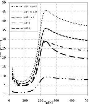
Figure 1 shows the WIP trends computed resorting to the three adopted models when TP changes from 20 to 500 hr. Curves referring to model I are shown for ce values of 0.5, 0.75, and 1. While significant differences in the computed values occur, due to the different approximations involved, all models show the same trend. In particular it is worth noting that two radically different models, namely Model III and Model I with ce = 0.5 show quite similar values. Model II show much lower WIP owing to the very low ce value resulting from the application of Hopp and Spearman model to the case of IFR, which raises doubts on the acceptability of this approximation. Overall, as TP is gradually increased, the WIP trend involves at first a rapid reduction until a minimum is reached, then an increase, followed by a final stabilization to an asymptotic value. This may be explained observing that, apart from the variability term, WIP directly depends from the resource saturation which, in turn, is directly dependent on the value of the effective process time. Figure 2 then shows the variation of effective process time. In Figure 2a), which refers to models I and II, we observe three distinct zones. In the first zone, for small values of TP, the value of te is high, but rapidly decreasing, because of the significant impact of preventive maintenance downtime. This downtime is distributed over a comparatively small number of pieces given the high frequency of preventive maintenance actions. Contribution of corrective maintenance downtime is instead negligible as the frequent preventive maintenance keeps the system failure rate low and few breakdowns are expected given that MTTF > TP. In the third zone, for high values of
TP, the contribution of preventive downtime becomes negligible, given that a high number of pieces are processed between preventive stoppages, and the corrective downtime contribution stabilizes to the value corresponding to distributing the corrective downtime over the average number of pieces processed between two consecutive breakdowns, given that TP becomes greater than MTTF and that for high TP values the frequency of preventive maintenance has only a negligible effect on the failure rate which stabilizes towards an asymptotic value. In the intermediate zone a minimum of te, and thus WIP, may occur or not depending on the trade-off between the competing effects of reducing preventive stoppages and increasing corrective stoppages, when TP and MTTF become comparable and changes in TP strongly affect MTTF variations and resource availability. Figure 2b) instead shows
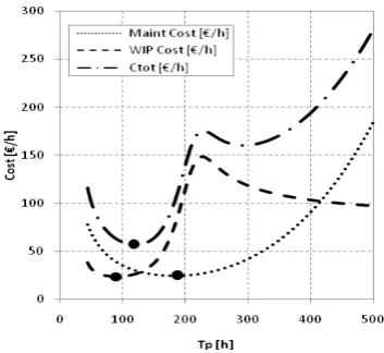
[image:5.595.358.502.542.710.2]te computed according to Model III where only the effect of corrective stoppages is included, being the preventive stoppages treated separately. In that figure the asymptotically stabilizing contribution of breakdowns is evident. Finally, Figure 2c) shows the trend of te computed with models I and II but in a different case respect that of Table I, showing that the above described trade-off between corrective and preventive downtime effects on effective process time does not necessarily give rise to a minimum value of te. Figure 3, shows instead the WIP curve of model III superimposed to the total maintenance cost per unit time CAU (TP) curves computed according to (6). Three curves are depicted for different couples of preventive and corrective intervention costs. This shows that while the actual costs involved in maintenance actions define a different optimal preventive maintenance interval, this interval is obviously not related to the interval minimizing WIP, and significant percent increases of WIP may occur when TP is set at the minimum maintenance cost respect the minimum WIP value. Therefore, if we sum to the overall maintenance cost CAU (TP), the WIP holding cost, CWIP(TP) = h WIP, where h (€/unit hr) is the unit WIP carrying cost, we can compute a total cost as shown in Figure 4. The corresponding TP value minimizing this total cost can be another option for planning a maintenance policy.
a) b) c) Figure 2. Trends of effective process time vs preventive maintenance interval
Figure 3. Trends of WIP and maintenance costs (legend: Cmp = CP, Cmg = CB).
Figure 4. Trends of WIP, maintenance and total costs. I. CONCLUSIONS
In this paper some queueing models have been used to assess the effects that the preventive maintenance interval has on the operational performance of single machine manufacturing systems characterized by an increased failure rate. While the study pointed out that still some research work is required to develop precise queueing models for unreliable servers undergoing both preemptive an non preemptive interruptions with non exponentially distributed uptimes, it was also shown that such approximate models can help to quickly represent the order of magnitude and the effects of the involved trade offs. In particular, it was shown that WIP can be very sensitive to the preventive maintenance interval, and that the minimum cost maintenance interval is not related to a minimum WIP. Arbitrary selection of this
interval or its choice made to minimize only the maintenance cost can have a detrimental effect on the system performances. Presented models allow, instead, to determine the maintenance interval giving the minimum total cost or, anyway, can help maintenance planners to make more informed decision related to costs-performances trade offs.
REFERENCES
[1] M.Ben-Daya, S.O. Duffuaa, A. Raouf, Maintenance, Modeling and Optimization, Springer, 2000.
[2] M.A. Crespo, The Maintenance Management Framework. Models and Methods for Complex Systems Maintenance, Springer, 2007.
[3] S.O. Duffuaa, A. Raouf, J.D. Campbell, Planning and Control of Maintenance Systems: Modeling and Analysis, Wiley, 1998.
[4] T. Nakagawa, Maintenance Theory of Reliability, Springer, 2005. [5] H. Wang, “A survey of maintenance policies of deteriorating systems,”
European Journal of Operational Research, Vol. 139, pp. 469-489, 2002.
[6] D. Gupta, Y. Günalay, M.M. Srinivasan, “The relationship between preventive maintenance and manufacturing systems performance,”
European Journal of Operational Research, Vol. 132, pp. 146-162, 2001.
[7] S.M.R. Iravani, I. Duenyas, “Integrated maintenance and production control of a deteriorating production system,” IIE Transactions, Vol. 34, pp. 423-435, 2002.
[8] J.C. Ke, “The optimal control of an M/G/1 queueing system with server vacations, startup and breakdowns,” Computers & Industrial Engineering, Vol. 44, pp. 567-579, 2003.
[9] D. Perry, M.J.M. Posner, “A correlated M/G/1-type queue with randomized server repair and maintenance modes,” Operations Research Letters, Vol. 26, pp. 137-147, 2000.
[10] C.E. Ebeling, An Introduction to Reliability and Maintainability Engineering, McGraw Hill, 1997.
[11] D. Gross, J.F. Shortle, J.M. Thompson, C.M. Harris, Queueing Theory, Wiley, 2008.
[12] T. Altiok, Performance Analysis of Manufacturing Systems, Springer, 1996.
[13] J.A. Buzacott, G. Shantikumar, Stochastic Models of Manufacturing Systems, Prentice Hall, 1993.
[14] R. Suri, J.L. Sanders, M. Kamath, “Performance evaluation of production networks,” in Graves, S.C.et al. (Ed.), Handbook of Operations research & Management Science, Vol. 4, pp. 199-286, 1993. [15] B. Avi-Itzhak, P. Naor, “Some queueing problems with service station subject to server breakdown,” Operations Research, Vol. 10, pp. 303-320, 1962.
[16] A. Federgruen, L. Green, “Queueing systems with service interruptions,” Operations Research, Vol. 34, No. 5, pp. 752-768, 1986. [17] H.C. White, L.S. Christie, “Queueing with preemptive priorities or with
breakdowns,” Operations Research, Vol. 6, pp. 79-95, 1958.
[18] K. Wu, L.F. McGinnis, B. Zwart, “Queueing models for single machine manufacturing systems with interruptions,” Proc. 2008 Winter Simulation Conference, IEEE, pp. 2083-2092.
[19] W.Whitt, “Approximations for the GI/G/m queue,” Production and Operations Management, Vol. 2, pp. 114-161, 1993
[20] W.J. Hopp, M.L. Spearman, Factory Physics, McGraw Hill, 2000. [21] I. Adan, J. Resing, Queueing Theory, Lecture Notes. Available:
http://www.win.tue.nl/~iadan/queueing.pdf.
[22] J.D.C. Little, “A Proof of the queueing formula: L = λW,” Operations Research, Vol. 9, pp. 383-387, 1961.
[image:6.595.78.255.405.567.2]