Abstract—This research involves a thermodynamic approach
to modeling and power optimization of nonlinear energy converters, such like thermal, solar and chemical engines. Thermodynamic principles lead to converter’s efficiency and limiting generated power. Efficiency equations serve to solve problems of upgrading and downgrading of a resource medium. Real work yield is a cumulative effect obtained in a system of a resource fluid, engines, and an infinite bath. While optimization of steady systems requires using of differential calculus and Lagrange multipliers, dynamic optimization involves variational calculus and dynamic programming. The primary result of the static optimization is the limiting value of power, whereas that of the dynamic optimization (treated here with a particular care) is a finite-rate counterpart of the classical potential of reversible work (exergy). This generalized potential depends on thermal coordinates and a dissipation index, h, i.e. the Hamiltonian of the related problem of minimum entropy production. The generalized potential implies stronger bounds on work delivered or supplied than the reversible work potential. In reacting systems the chemical affinity constitutes a prevailing counterpart of the thermal efficiency. Therefore, in reacting mixtures flux balances are applied to derive power yield in terms of an active part of chemical affinity.
Index Terms—Keywords. Resources, thermal efficiency,
chemical efficiency, entropy production, engines.
I. INTRODUCTION
Applications of thermodynamics of finite rates lead to solutions which describe various forms of bounds on power and energy production (consumption) including in dynamical cases finite-rate generalizations of the standard availabilities. In this research we treat power limits in static and dynamical energy systems driven by nonlinear fluids that are restricted in their amount or magnitude of flow, and, as such, play role of resources. A power limit is an upper (lower) bound on power produced (consumed) in the system. A resource is a valuable substance or energy used in a process; its value can be quantified by specifying its exergy, a maximum work that can be obtained when the resource relaxes to the equilibrium. Reversible relaxation of the resource is associated with the classical exergy. When dissipative phenomena prevail generalized exergies are essential. In fact, generalized exergies quantify deviations of the system’s efficiency from the Carnot efficiency. An exergy is obtained as the principal component of solution to the variational problem of
Manuscript received December 1, 2008. This research was supported by the grant: Thermodynamics and Optimization of Chemical and Electrochemical Energy Generators with Applications to Fuel Cells, nr N N208 019434, from Polish Ministry of Science. S. Sieniutycz is with the Faculty of Chemical and Process Engineering at Warsaw TU, 1 Waryńskiego Street, Warszawa, 00645 Poland (phone: 00-48228256340; fax: 00-48228251440; e-mail: sieniutycz@ ichip.pw.edu.pl).
extremum work under suitable boundary conditions. Other components of the solution are optimal trajectory and optimal control. In purely thermal systems (those without chemical changes) the trajectory is characterized by temperature of the resource fluid, T(t), whereas the control is Carnot temperature T’(t) defined in our previous work [1, 2]. For chemical systems also chemical potential(s) μ’(t) plays a role. Whenever T’(t) and μ’(t) differ from T(t) and μ(t) the resource relaxes with a finite rate, and with an efficiency vector different from the perfect efficiency. Only when T’ = T and μ’= μ the efficiency is pefect, but this corresponds with an infinitely slow relaxation rate of the resource to the thermodynamic equilibrium with the environmental fluid.
The structure of this paper is as follows. Section II discusses various aspects power optimization. Properties of steady systems are outlined in Sec. III, whereas those of dynamical ones - in Sec. IV. Section V develops quantitative analyses of resource downgrading (in the first reservoir) and outlines properties of generalized potentials for finite rates. Sections VI-VIII discuss various Hamilton-Jacobi-Bellman equations (HJB equations) for optimal work functions, as solutions of power yield problems. Extensions for simple chemical systems are outlined in Sec. IX.
The size limitation of our paper does not allow for inclusion of all derivations to make the paper self-contained, thus the reader may need to turn to some previous works, [1] - [5]. In view of difficulties in getting analytical solutions in complex systems, difference equations and numerical approaches are treated in ref. [3] which also discusses convergence of numerical algorithms to solutions of HJB equations and role of Lagrange multipliers in the dimensionality reduction.
II. FINITE RESOURCES AND POWER OPTIMIZATION Limited amount or flow of a resource working in an engine causes a decrease of the resource potential in time (chronological or spatial). This is why studies of the resource downgrading apply the dynamical optimization methods. From the optimization viewpoint, dynamical process is every one with sequence of states, developing either in the chronological time or in (spatial) holdup time. The first group refers to unsteady processes in non-stationary systems, the second group may involve steady state systems.
In a process of energy production two resting reservoirs do interact through an energy generator (engine). In this process power flow is steady only when two reservoirs are infinite. When one, say, upper, reservoir is finite, its thermal potential must decrease in time, which is consequence of the energy balance. Any finite reservoir is thus a resource reservoir. It is the resource property that leads to the dynamical behavior of the fluid and its relaxation to the equilibrium with an infinite
Maximization of Power Yield in Thermal and
Chemical Systems
lower reservoir (usually the environment).
Alternatively, fluid at a steady flow can replace resting upper reservoir. The resource downgrading is then a steady-state process in which the resource fluid flows through a pipeline or stages of a cascade and the fluid’s state changes along a steady trajectory. As in the previous case the trajectory is a curve describing the fluid’s relaxation towards the equilibrium between the fluid and the lower reservoir (the environment). This is sometimes called “active relaxation” as it is associated with the simultaneous work production. It should be contrasted with “dissipative relaxation”, a well-known, natural process between a body or a fluid and the environment without any power production.
Relaxation (either active or dissipative) leads to a decrease of the resource potential (i.e. temperature) in time. An inverse of the relaxation process is the one in which a body or a fluid abandons the equilibrium. This cannot be spontaneous; rather the inverse process needs a supply of external power. This is the process referred to thermal upgrading of the resource, which can be accomplished with a heat pump.
III. STEADY SYSTEMS
The great deal of research on power limits published to date deals with stationary systems, in which case both reservoirs are infinite. To this case refer steady-state analyses of the Chambadal-Novikov-Curzon-Ahlborn engine (CNCA engine [6]), in which energy exchange is described by Newtonian law of cooling, or the Stefan-Boltzmann engine, a system with the radiation fluids and the energy exchange governed by the Stefan-Boltzmann law [7]. Due to their stationarity (caused by the infiniteness of both reservoirs), controls maximizing power are lumped to a fixed point in the state space. In fact, for the CNCA engine, the maximum power point may be related to the optimum value of a free (unconstrained) control variable which can be efficiency η or Carnot temperature T’. In terms of the reservoirs temperatures T1 and T2 and the internal irreversibility factor
Φ one finds 12
2 1 =
′ (TΦT ) /
Topt [4]. For the Stefan-Boltzmann
[image:2.595.100.240.611.740.2]engine exact expression for the optimal point cannot be determined analytically, yet, this temperature can be found graphically from the chart P=f(T’).
Figure 1. Maximum power relaxation curve for black radiation without constraint on the temperature [8].
Moreover, the method of Lagrange multipliers can successfully be applied [8]. As their elimination from a set of resulting equations is quite easy, the problem is broken down to the numerical solving of a nonlinear equation for the optimal control T’. Finally, the so-called pseudo-Newtonian model [4, 5], which uses state or temperature dependent heat exchange coefficient, α(T3), omits, to a considerable extent,
analytical difficulties associated with the Stefan-Boltzmann equation. Applying this model in the so-called symmetric case, where both reservoirs are filled up with radiation, one shows that the optimal (power maximizing) Carnot temperature of the steady radiation engine is that for the CNCA engine, i.e. [4]. This equation is, in fact, a good approximation under the assumption of transfer coefficients dependent solely on bulk temperatures of reservoirs.
IV. DYNAMICAL SYSTEMS
The evaluation of dynamical energy yield requires the knowledge of an extremal curve rather than an extremum point. This is associated with application of variational metods (to handle functional extrema) in place of static optimization methods (to handle extrema of functions). For example, the use of the pseudo-Newtonian model to quantify the dynamical energy yield from radiation, gives rise to an extremal curve describing the radiation relaxation to the equilibrium. This curve is non-expotential, the consequence of the nonlinear properties of the relaxation dynamics. Non-expotential are also other curves describing the radiation relaxation, e.g. those following from exact models using the Stefan-Boltzmann equation (symmetric and hybrid, [4,5]).
Analytical difficulties associated with dynamical optimization of nonlinear systems are severe; this is why diverse models of power yield and diverse numerical approaches are applied. Optimal (e.g. power-maximizing) relaxation curve T(t) is associated with the optimal control curve T’(t); they both are components of the dynamic optimization solution to a continuous problem. In the corresponding discrete problem, formulated for numerical purposes, one searches for optimal temperature sequences {Tn} and {T’n}. Various discrete optimization methods
involve: direct search, dynamic programming, discrete maximum principle, and combinations of these methods.
Minimum power supplied to the system is described in a suitable way by function sequences Rn(Tn, tn), whereas
maximum power produced – by functions Vn(Tn, tn).
Profit-type performance function V and cost-type performance function R simply differ by sign, i.e. Vn(Tn, tn) =
- Rn(Tn, tn). The beginner may find the change from symbol V
to symbol R and back as unnecessary and confusing. Yet, each function is positive in its own, natural regime of working (V - in the engine range and R - in the heat pump range).
generalized exergies. The latter depend not only on classical thermodynamic variables but also on their rates. These generalized exergies refer to state changes in a finite time, and can be contrasted with the classical exergies that refer to reversible quasistatic processes evolving in time infinitely slowly. The benefit obtained from generalized exergies is that they define stronger energy limits than those predicted by classical exergies. Systematic approach to exergies (classical or generalized) based on work functionals leads to several original results in thermodynamics of energy systems, in particular it allows to explain unknown properties of exergy of black-body radiation or solar radiation, and to show that the efficiency of the solar energy flux transformation is equal to the Carnot efficiency.
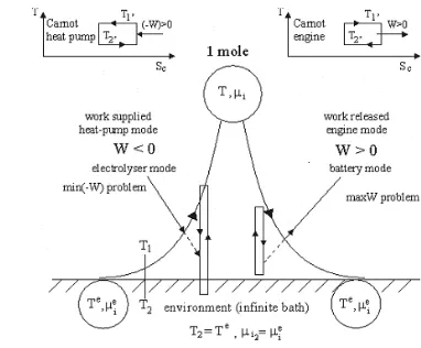
V. TWO WORKS AND FINITE-TIME EXERGY
Two different works, the first associated with the resource downgrading during its relaxation to the equilibrium and the second – with the reverse process of resource upgrading, are essential (Fig.2). During the approach to the equilibrium engine mode takes place in which work is released, during the departure- heat-pump mode occurs in which work is supplied. Work W delivered in the engine mode is positive by assumption (“engine convention”). Sequence of irreversible engines (CNCA or Stefan-Boltzmann) serves to determine a rate-dependent exergy extending the classical exergy for irreversible, finite rate processes. Before maximization of a work integral, process efficiency η has to be expressed as a function of state T and a control, i.e. energy flux q or rate dT/dτ, to assure the functional property (path dependence) of the work integral. The integration must be preceded by maximization of power or work at flow (the ratio of power and flux of driving substance) w to assure an optimal path. The optimal work is sought in the form of a potential function that depends on the end states and duration. For appropriate boundary conditions, the principal function of the variational problem of extremum work coincides with the notion of an exergy, the function that characterizes quality of resources.
[image:3.595.72.263.536.694.2]
Figure 2. Two works: Limiting work produced and limiting work consumed are different in an irreversible process.
The idea of an infinite number of infinitesimal CNCA steps, necessary for exergy calculations, is illustrated in Fig.2. Each step is a work-producing (consuming) stage with
the energy exchange between two fluids and the thermal machine through finite“conductances”. For the radiation engine it follows from the Stefan-Boltzmann law that the effective transfer coefficient α1 of the radiation fluid is
necessarily temperature dependent, α1= ∝T13. The second or
low-T fluid represents the usual environment, as defined in the exergy theory. This fluid possesses its own boundary layer as a dissipative component, and the corresponding exchange coefficient is α2. In the physical space, the flow
direction of the resource fluid is along the horizontal coordinate x. The optimizer’s task is to find an optimal temperature of the resource fluid along the path that extremizes the work consumed or delivered.
Total power obtained from an infinite number of infinitesimal engines is determined as the Lagrange functional of the following structure
∫
∫
′ =− ′= 0
f
i f
i
t
t t
t f
i f T T dt GcT ηT T Tdt
W[T ,T ] ( , ) ( ) ( , ) (1)
where f0 is power generation intensity, G - resource flux,
c(T)-specific heat, η(T, T’)-efficiency in terms of state T and control T, further T– enlarged state vector comprising state and time, t –time variable (residence time or holdup time) for the resource contacting with heat transfer surface. Sometimes one uses a non-dimensional time τ, identical with the so-called number of the heat transfer units. Note that, for constant mass flow of a resource, one can extremize power per unit mass flux, i.e. the quantity of work dimension called “work at flow”. In this case Eq. (1) describes a problem of extremum work. Integrand f0 is common for both modes, yet
the numerical results it generates differ by sign (positive for engine mode; “engine convention”). When the resource flux is constant a work functional describing the thermal exergy flux per unit flux of resource can be obtained from Eq. (1)
dT dT dt T T
T T
c w
f e
i
T T
T T
e
dt dT
∫
=
= ⎟⎟⎠
⎞ ⎜⎜
⎝ ⎛
′ − −
=
) / , ( 1 ) ( /
max . (2)
Note that the independent variable in this equation is T, i.e. it is different than that in Eq. (1).
The function f0 in Eq. (1) contains thermal efficiency
function, η, described by a practical counterpart of the Carnot formula. When T > Te, efficiency η decreases in the engine
mode above ηC and increases in the heat-pump mode below
ηC. At the limit of vanishing rates, dT/dt = 0 and T′→T.
Then work of each mode simplifies to the common integral of the classical exergy. For the classical thermal exergy
) ( 1
) ( 0
/ max
e e e T
T
T T
e
dt dT
s s T h h dT T T T c w
f e
i
− − − = ⎟⎟ ⎠ ⎞ ⎜⎜ ⎝ ⎛
− −
= =∫ = →
.
(3) Nonlinearities can have both thermodynamic and kinetic origins; the former refer, for example, to state dependent heat capacity, c(T), the latter to nonlinear energy exchange. Problems with linear kinetics (Newtonian heat transfer) are an important subclass. In problems with linear kinetics, fluid’s specific work at flow, w, is described by an equationdτ
T T
T T T c T dT T T T c G W w
f
i f
i
t
t e T
T
e f
i
′ − ′ −
⎟ ⎟ ⎠ ⎞ ⎜ ⎜ ⎝ ⎛
− 1 − =
= /
∫
( )∫
( )( )2]
[T,T
(4)
χ α
α
τ t t
c G Fv a x c G F a H
x v v
TU = ′ = ′ =
≡
(5)
is non-dimensional time of the process. Equation (5) assumes that a resource fluid flows with velocity v through cross-section F and contacts with the heat transfer exchange surface per unit volume av [1]. Quantity τ is identical with the
so-called number of the heat transfer units.
Solutions to work extremum problems can be obtained by: a) variational methods, i.e. via Euler-Lagrange equation of variational calculus 0 = ⎟ ⎠ ⎞ ⎜ ⎝ ⎛ ∂ ∂ − ∂ ∂ T L dt d T L
.
(6) In the example considered above, i.e. for a thermal system with linear kinetics
⎟ =0
⎠ ⎞ ⎜ ⎝ ⎛ τ − τ 2 2 2 d dT d T d
T
(7)
which corresponds with the optimal trajectory f i f i f i
f T T T T T
T(τ,τ , , )= ( / )τ/τ . (8)
(τi =0 is assumed in Eq. (8).) However, the solution of
Euler-Lagrange equation does not contain any information about the optimal work function. This is assured by solving the Hamilton-Jacobi-Bellman equation (HJB equation, [9]). b) dynamic programming via HJB equation for the ‘principal function’ (V or R), also called extremum work function. For the linear kinetics considered
0 ) ))( 1 ( ( max = ⎭ ⎬ ⎫ ⎩ ⎨ ⎧ − ′ ′ − − ∂ ∂ − − ∂ ∂
′ T T T
T c T V V e T
τ . (9)
Observe that all rates (f0 and f) and derivatives of V are
evaluated at the final state (the so-called ‘forward equation’). The extremal work function V is a function of the final state and total duration. After evaluation of optimal control and its substitution to Eq. (9) one obtains a nonlinear equation
{
− (1+ 1∂ /∂ )}
2=0− ∂
∂V c Te T c− V T
τ . (10)
which is the Hamilton-Jacobi equation of the problem. Its solution can be found by the integration of work intensity along an optimal path, between limits Ti and Tf. A reversible
(path independent) part of V is the classical exergy A(T, Te,
0).
Details of models of multistage power production in sequences of infinitesimal engines are known from previous publications [1]-[5]. These models provide power generation functions f0 or thermal Lagrangians l0 = -f0 and dynamical
constraints. Numerical methods apply suitable discrete models, for given rates f0 and f. An important issue is
convergence of these discrete models to continuous ones [3].
VI. HJB EQUATIONS FOR NONLINEAR POWER SYSTEMS We shall display here some Hamilton-Jacobi-Bellman equations for power systems described by nonlinear kinetics. A suitable example is a radiation engine whose power integral is approximated by a pseudo-Newtonian model of radiative energy exchange associated with optimal function
⎟⎟ ⎠ ⎞ ⎜⎜ ⎝ ⎛ ′ ′ ′ − − ≡ ∫ f i t t e m m t T f f i
i υ T T dt
T T Φ c G t T t T
V( , , , ) max (1 ) ( , )
) ('
(11)
where υ =α(T3)(T’-T). An alternative form uses Carnot
temperature T’ explicit in υ [5]. Optimal power (11) can be referred to the integral
dt T T T c T c G W T T e vm hm m υ
∫
⎟⎟ ⎠ ⎞ ⎜⎜ ⎝ ⎛ − −= 0 ( ) ( )
dt T Φ T T T c G T m vm T T e ⎟ ⎟ ⎠ ⎞ ⎜ ⎜ ⎝ ⎛ χυ + υ − 1 + χυ + χυ
−
∫
20 ) ( ( ) ) ( ) (
. (12)
This process is described by a pseudolinear kinetics dT/dt = f(T, T’) consistent with υ =α(T3)(T’-T) and a general form
of HJB equation for work function V is 0 ) , ( ) , ( max 0 ) ( ⎟⎠= ⎞ ⎜ ⎝ ⎛ ′ ∂ ∂ − ′ + ∂ ∂ −
′ T f T T
V T T f t V t T
. (13)
where f0 is defined as the integrand of Eq. (11) or (12).
A more exact model or radiation conversion relaxes the assumption of the pseudo-Newtonian transfer and applies the Stefan-Boltzmann law. For a symmetric model of radiation conversion (both reservoirs composed of radiation)
dt T T T Φ T T T ΦT T G W f i t
t e a a
a a e
c
∫
′ ′ −1+1 −1′ − β ⎟ ⎟ ⎠ ⎞ ⎜ ⎜ ⎝ ⎛ ′ − 1 = ) ) / ( ( ) (
. (14)
The coefficient is = −1( 0)−1
m h vc p
a
σ
β is related to molar
constant of photons density 0 m
p and Stefan-Boltzmann constant σ. In the physical space, power exponent a=4 for radiation and a=1 for a linear resource. With state equation
1 1 1)
) / ( ( ′ ′ − + − ′ − −
= ae a a a
T T T Φ T T dt
dT β (15)
[5] applied in general Eq. (19) we obtain a HJB equation
0 ) 1 ) / ( ( / ) 1 (
max 1 1
2 ) ( ⎪= ⎭ ⎪ ⎬ ⎫ ⎪ ⎩ ⎪ ⎨ ⎧ + ′ ′ ′ − ⎟ ⎟ ⎟ ⎠ ⎞ ⎜ ⎜ ⎜ ⎝ ⎛ ∂ ∂ + ′ − + ∂ ∂ − − −
′ a a
a a e
c t
T Φ T T T
T T T V T T Φ G t
V β (16)
Dynamics (15) is the characteristic equation for Eq. (16). For a hybrid model of radiation conversion (upper reservoir composed of the radiation and lower reservoir of a Newtonian fluid, [5]) the power is
udt g ug T Φ u T T ΦT T G
W a a a e a
t c f i ⎟ ⎟ ⎠ ⎞ ⎜ ⎜ ⎝ ⎛ β + β + − 1 − = 2 1 1 − 1 − 1 1 − 1 −
τ
∫
( ) /)
( /
(17) and the corresponding Hamilton-Jacobi-Bellman equation is
0 ) / ) ( 1 )( ( max 2 1 1 1 / 1 1 1 ) ( = ⎪ ⎭ ⎪ ⎬ ⎫ ⎪ ⎩ ⎪ ⎨ ⎧ ⎟ ⎟ ⎟ ⎠ ⎞ ⎜ ⎜ ⎜ ⎝ ⎛ ∂ ∂ + + + − − + ∂ ∂ − − − − − ′ u T V g ug T Φ u T T ΦT T G t V f a a a a e c t T f β β (18)
VII. ANALYTICAL ASPECTS OF LINEAR AND PSEUDO-NEWTONIAN KINETICS
driving temperature T' or other control is implemented as the quantity maximizing the hamiltonian with respect to T’ at each point of the path. The maximization of H leads to two equations. The first expresses optimal control T' in terms of T and z = - ∂V/∂T. For the linear kinetics of Eq. (9) we obtain
0 ) 1 ( ) , ( 2 0 = ′ − + ∂ ∂ = ′ ∂ ′ ∂ − ∂ ∂ T T T c T V T T T f T V e (19) whereas the second is the original equation (9) without maximizing operation 0 ) )( 1 ( )
( 2 ′− =
′ − + − ′ ∂ ∂ + ∂
∂ T T
T T c T T T V V
τ (20)
To obtain optimal control function T'(z, T) one should solve the second equality in equation (19) in terms of T', The result is Carnot control T' in terms of T and z = - ∂V/∂T,
2 / 1
1 /
1 ⎟⎟⎠
⎞ ⎜⎜ ⎝ ⎛ ∂ ∂ + = ′ − T V c T T
T e . (21)
This is next substituted into (20); the result is the nonlinear Hamilton-Jacobi equation
(
1+ 1∂ /∂ − /)
2 =0 +∂ ∂
− V cT c− V T Te T
τ (22)
which contains the energylike (extremum) Hamiltonian of the extremal process.
(
)
21 / /
1 )
,
( cT c V T T T
T V T
H = + ∂ ∂ − e
∂
∂ − . (23)
For a positively-defined H, each Hamilton-Jacobi equation for optimal work preserves the general form of autonomous equations known from analytical mechanics and theory of optimal control.
Expressing extremum Hamiltonian (23) in terms of state variable T and Carnot control T ' yields an energylike function satisfying the following relations
2 2 0 0 ) ( ) , ( T T T cT u f u f u T E e ′ − ′ = ∂ ∂ −
= (24)
E is the Legendre transform of the work lagrangian l0 = - f0
with respect to the rate u = dT/dτ .
Assuming a numerical value of the Hamiltonian, say h, one can exploit the constancy of H to eliminate ∂V/∂T. Next combining equation H=h with optimal control (21), or with an equivalent result for energy flow control u=T ‘-T
T T V c T T u e − ⎟⎟ ⎠ ⎞ ⎜⎜ ⎝ ⎛ ∂ ∂ + = − 2 / 1 1 /
1 . (25)
yields optimal rate u=Tin terms of temperature T and the Hamiltonian constant h
T cT h cT
h
T={± / e(1−± / e)−1}
(26) A more general form of this result which applies to systems with internal dissipation (factor Φ) and applies to the pseudo-Newtonian model of radiation is
T T Φ T T Φc T Φc T v v ) , , ( ) ( 1 ) ( 1 σ σ
σ h ξ h
h ≡ ⎟⎟ ⎟ ⎠ ⎞ ⎜⎜ ⎜ ⎝ ⎛ ⎟ ⎟ ⎠ ⎞ ⎜ ⎜ ⎝ ⎛ ± − ± = −
(27)
where ξ , defined in the above equation, is an intensity index and hσ=h/T. This result is obtained by the application of
variational calculus to nonlinear radiation fluids with the temperature dependent heat capacity cv(T)=4a0T3. Positive ξ
refer to heating of the resource fluid in the heat-pump mode, and the negative - to cooling of this fluid in the engine mode. Thus pseudo-Newtonian systems produce power relaxing with the optimal rate
T
Φ
T h
T=
ξ
( σ, , ) . (28) Equations (27) and (28) describe the optimal trajectory in terms of state variable T and constant h. The corresponding optimal (Carnot) control is(
ΦT)
TT′= 1+ξ(hσ, , ) (29) The presence of resource temperature T in function ξ proves that, in comparison with the linear systems, the pseudo-Newtonian relaxation curve is not exponential.
VIII. OPTIMAL WORK FUNCTIONS FOR LINEAR AND PSEUDO-NEWTONIAN KINETICS
A solution can now be found to the problem of Hamiltonian representation of extremal work. Let us begin with linear systems. Substituting temperature control (29) with a constant ξ into work functional (4) and integrating along an optimal path yields extremal work function
f i e e f i e f i f i T T cT h cT T T cT T T c h T T
V( , , )= ( − )− ln − ln (30)
This expression is valid for every process mode. Integration of Eq (27) subject to end conditions T(τi)=Ti and T(τf)=Tf
allows to express Eq. (30) in terms of the process duration. For the radiation cv(T)=4a0T3, where a0 is the radiation
constant, an optimal trajectory solving Eqs. (27) and (29) is
i i
i T T τ
T T
Φ
a ⎜⎝⎛ − ⎟⎠⎞− = −τ
3 4
±( / ) 012 12 σ 32 32 ln( / ) / / 2 / 1 -/ / h (31) The integration limits refer to the initial state (i) and a current state of the radiation fluid, i.e. temperatures Ti and T
corresponding with τi and τ. Optimal curve (31) refers to the
case when the radiation relaxation is subject to a constraint resulting from Eq. (28).
Equation (31) is associated with the entropy production term in Eq. (12). The corresponding extremal work function per unit volume of flowing radiation is
) )( 1 ( ) 3 / 4 ( ) ( ) 3 / 4 ( ) ( 3 3 0 2 / 3 2 / 3 2 / 1 2 / 1
0 e i f e i f
f v i v e f v i v T T Φ T a T T T Φ a s s T h h V − − + − − − − − ≡ 1/2 hσ (32)
Also, the corresponding exergy function, obtained from (32) after applying exergy boundary conditions, has an explicit analytical form. The classical availability of radiation at flow resides in the resulting exergy equation in Jeter’s [10] form
) / 1 ( ) 3 / 4 ( ) / 1 ( ) ( ) 0 , , ( 4
0T T T
a T T h s s T h h T T A e e v e v v e e v v e class v − = − = − − −
= . (33)
participate in transformation of chemical affinities into mechanical power [11]. Yet, as opposed to thermal machines, in chemical ones generalized reservoirs are present, capable of providing both heat and substance. When infinite reservoirs assure constancy of chemical potentials, problems of extremum power (maximum of power produced and minimum of power consumed) are static optimization problems. For finite reservoirs, however, amount and chemical potential of an active reactant decrease in time, and considered problems are those of dynamic optimization and variational calculus. Because of the diversity and complexity of chemical systems the area of power producing chemistries is extremely broad. The simplest model of power producing chemical engine is that with an isothermal and isomeric reaction, A1+A2=0 [11]. Power expression and efficiency
formula for the chemical system follow from the entropy conservation and energy balance in the power-producing zone of the system (active part). In “endoreversible chemical engines” the total entropy flux is continuous through the active zone. When a formula describing this continuity is combined with energy balance we find in an isothermal case
n
p=(μ1'−μ2') (34)
where n is an invariant molar flux of reagents. Process efficiency ζ is defined as power yield per molar flux, n, i.e.
' 2 ' 1
/ μ μ
ζ = p n= − (35) This efficiency is identical with the chemical affinity of our reaction in the chemically active part of the system. While ζ is not dimensionless, it describes correctly the system.
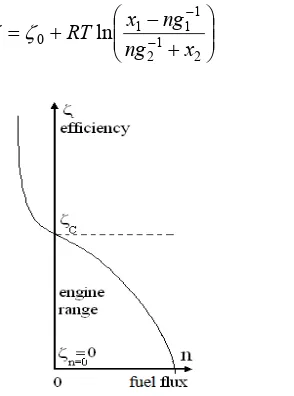
For a steady engine the following function defines the chemical efficiency in terms of n and mole fraction x (Fig. 3)
⎟⎟ ⎠ ⎞ ⎜⎜
⎝ ⎛
+ − +
= − −
2 1 2
1 1 1 0 ln ng x
ng x RT
ζ
[image:6.595.109.256.477.675.2]ζ (36)
Figure 3. Efficiency of power production ζin terms of fuel flux n in a chemical engine.
Equation (36) shows that an effective concentration of the reactant in upper reservoir x1eff = x1 – g1-1n is decreased,
whereas an effective concentration of the product in lower reservoir x2eff = x2 + g2-1 n is increased due to the finite mass
flux. Therefore efficiency ζ decreases nonlinearly with n.
When effect of resistances −1 k
g is ignorable or flux n is very small, reversible efficiency, ζC, is attained. The power
function, described by the product ζ(n)n, exhibits a maximum for a finite value of the fuel flux, n.
Application of Eq. (36) to an unsteady system leads to a work function describing the dynamical limit of the system
1 1 1
2
1
0 /
/ ) 1 /( ln 1
1
τ τ τ
τ ζ
τ
τ
d d dX d
jdX x
d dX X X RT W
f
i ⎭
⎬ ⎫ ⎩
⎨ ⎧
⎟⎟ ⎠ ⎞ ⎜⎜
⎝ ⎛
− + + +
−
=
∫
(37)(X=x/(1-x).) The path optimality condition may be expressed in terms of the constancy of the following Hamiltonian
⎟⎟ ⎠ ⎞ ⎜⎜
⎝ ⎛
+ + =
+ =
2 2
2 1
1 2
2 1
) (
) ( )
, (
x j X
X X RT x X x
X jx x X RT X X
H . (38)
For low rates and large concentrations X (mole fractions x1 close to the unity) optimal relaxation rate is approximately
constant. Yet, in an arbitrary situation optimal rates are state dependent so as to preserve the constancy of H in Eq. (38).
Extensions of Eq. (36) are available for multicomponent and multireaction systems [12].
REFERENCES
[1] S. Sieniutycz, “A synthesis of thermodynamic models unifying traditional and work-driven operations with heat and mass exchange”,
Open Sys. & Information Dynamics, 10 (2003), 31-49..
[2] S. Sieniutycz, “Carnot controls to unify traditional and work-assisted operations with heat & mass transfer”, International J. of Applied Thermodynamics, 6 (2003), 59-67.
[3] S. Sieniutycz, “Dynamic programming and Lagrange multipliers for active relaxation of fluids in non-equilibrium systems”, Applied Mathematical Modeling, 33 (2009), 1457-1478.
[4] S. Sieniutycz and P. Kuran, “Nonlinear models for mechanical energy production in imperfect generators driven by thermal or solar energy”,
Intern. J. Heat Mass Transfer, 48 (2005), 719-730.
[5] S. Sieniutycz and P. Kuran, “Modeling thermal behavior and work flux in finite-rate systems with radiation”, Intern. J. Heat and Mass Transfer 49 (2006), 3264-3283.
[6] F.L. Curzon and B. Ahlborn, “Efficiency of Carnot engine at maximum power output”, American J. Phys. 43 (1975), 22-24.
[7] A. de Vos, Endoreversible Thermodynamics of Solear Energy Conversion, Oxford University Press, Oxford, 1994, pp.30-41. [8] P. Kuran, Nonlinear Models of Production of Mechanical Energy in
Non-Ideal Generators Driven by Thermal or Solar Energy, PhD thesis, Warsaw University of Technology, 2006.
[9] R. E. Bellman, Adaptive Control Processes: a Guided Tour, Princeton, University Press, 1961, pp.1-35.
[10] J. Jeter, “Maximum conversion efficiency for the utilization of direct solar radiation”, Solar Energy 26 (1981), 231-236.
[11] S. Sieniutycz, “An analysis of power and entropy generation in a chemical engine,” Intern. J. of Heat and Mass Transfer 51 (2008) 5859–5871.
![Figure 1. without constraint on the temperature [8]. Maximum power relaxation curve for black radiation](https://thumb-us.123doks.com/thumbv2/123dok_us/1314208.661604/2.595.100.240.611.740/figure-constraint-temperature-maximum-power-relaxation-curve-radiation.webp)