d((x, y), (a, b)) is the distance function that measure

Abstract—This paper describes the reinforcement learning (RL) algorithm for the minimal consistent subset identification (MCSI) problem. MCSI is widely used in pattern recognition to select prototypes from a training set to be used in nearest neighbor classification. The RL agent solves the MCSI problem by deselecting a prototype one by one from the original data set to search for the best subset. Because the algorithm rarely descends to the smaller solution via its exploration strategy, a simple modification to the algorithm is proposed. The modification encourages the agent to try as many actions as possible at the current best solution to improve the results obtained. The paper concludes by comparing the performance of the proposed algorithm in handling the MCSI problem with the RL algorithm and the standard MCSI method.

Index Terms—minimal consistent subset, nearest neighbor rule, prototype selection, reinforcement learning.

I. INTRODUCTION

Minimal consistent subset identification (MCSI) is the problem of selecting a minimum number of prototypes from training data set while maintaining the consistency property [2]. The set of prototypes selected can be used in the nearest neighbor classification [1] instead of using the original set. The selected prototype set is defined to be consistent if it is able to correctly classify the original data set by using the nearest neighbor classification.

The MCSI problem is a hard combinatorial problem [5] that the optimum solution cannot be found by fully exploring the search space in limited time. The traditional MCSI method [3] by Dasarathy is one of the prototype selection methods that try to obtain the minimal consistent subset. The drawback of the method is that it employs the greedy strategy and is usually being trapped in a local minimum. This paper investigates the alternative solution by applying the reinforcement learning (RL) [4] to the MCSI problem. The standard RL method is also being trapped in a local minimum. In order to escape from the local minimum, a simple modification to the RL algorithm is proposed. The key modification is the new definition of the state transition function. This enables the agent to try as many actions as possible from the potential state and prevents the agent from exploring the unproductive region.

Manuscript received August 13, 2009.

Ekaphol Anantapornkit is with the Department of Computer Engineering, Faculty of Engineering, King Mongkut`s Institute of Technology Ladkrabang, Bangkok, Thailand (e-mail: ekreal@yahoo.com).

Boontee Kruatrachue is with the Department of Computer Engineering, Faculty of Engineering, King Mongkut`s Institute of Technology Ladkrabang, Bangkok, Thailand (e-mail: booontee@yahoo.com).

This paper is organized into 6 sections. The nearest neighbor classification is reviewed in section II. Section III reviews the minimal consistent set identification method by Dasarathy [3]. Section IV explains how to apply the reinforcement learning to the MCSI problem. Section V presents a modification to the RL algorithm to improve the results obtained. The experimental results are shown in section VI. Section VII is the conclusion.

II. NEAREST NEIGHBOR RULE

A prototype set ((x1, y1), c1), … , ((xn, yn), cn) is given,

where the (xi, yi) is the attribute value of the data point ith and

ci is the category of the data ith.

The unknown data ((a, b), z) can be classified as cnn, which

is the category of the prototype that is the nearest neighbor of (a, b). If d((x, y), (a, b)) is the distance function that measure the difference (x, y) and (a, b). The nearest neighbor of unknown at (a, b) is defined as follows:

(xnn, ynn) = min d((xi, yi), (a, b)) ; i = 1, 2, …, n (1)

III. MINIMAL CONSISTENT SET IDENTIFICATION METHOD

Minimal consistent set identification (MCSI) method is one of the condensing-selection prototype selection methods, which is based on the concept of covering defined by “NUN”, the Nearest Unlike Neighbor [3]. Any data point A is covered by any data point B which has the same class as A, as long as B is nearer to A than A’s NUN. Hence, A can be correctly classified, using nearest neighbor rule, to be the same class as B if B is selected as a prototype, as B is closer to A than A’s NUN.

Once a distance matrix among all the data in the training set is sorted and all NUNs of each data point are located, a list of data points covered by any point B, B cover set, can be constructed. The cover list of B includes any data point A that has B located closer to A than A’s NUN. The prototypes can be selected greedily incrementally by choosing a data point which has the largest cover list. Once that prototype is selected all the data point in that data cover list is covered (guarantee to be correctly classified) and that cover list is subtracted from all the cover lists. Then the data with the largest cover list is selected again as another prototype. The selection and subtraction process continues until all the cover lists are empty, which indicate the occurring of consistence property, where all the training data can be correctly classified by the selected prototypes.

The prototype set selected from the above algorithm is consistent but is still not minimal for two reasons. The first

Reinforcement Learning Algorithm for the

Minimal Consistent Subset Identification

one is the greedy order of the prototype selection which has no guarantee to minimal number of prototype. The second one is the inaccuracy of cover list calculation using NUN as boundary, since if the NUN is not selected as a prototype the cover lists can be expand. But before all prototypes are selected, it is safe to assume cover list boundary at NUN. To alleviate this problem, the prototypes selected are used again as boundary (instead of NUN) and the whole process is repeated until there is no change in the prototype set.

The MCSI Algorithm proceeds in the following steps. (as shown in Fig. 1)

1) Create a sorted distance table (c) among all data in the original prototype set (a).

2) Label all the NUN (Nearest Unlike Neighbor) by assumes that all the NUN are selected prototype (c).

3) Create a cover list for each prototype (d).

4) Select the prototype with maximum cover, and remove all the data in the covered list from all the cover lists (e).

5) Repeat step 4 until all the cover lists is empty and obtains all new selected prototypes (f)

6) Stop if the new selected prototypes from step 5 are the same as the previous one.

7) Re-Label the sorted distance table (g) with the new selected prototypes from step 5.

8) Go to step 3.

The “cover” concept is shown in Fig. 1 (c), (d), where A1 covers A1, A2, A3 since A1 is closer to A1, A2 and A3 than B2, B2 and B1 (the nearest unlike neighbor of A1,A2 and A3). Hence, if A1 is selected as a prototype, A1, A2 and A3 can be correctly recognized.

(a) Original prototype set. (b) Distance table.

(c) 1st sorted and labeled distance table.

(d) 1st selection. (e) 2nd selection. (f) 3rd selection.

(g) Re-labeled sorted distance table. Fig. 1 Illustration of the MCSI algorithm

From Fig. 1, the first round of the MCSI obtains A1, A4, and B1 as a prototype set. After the second round, the MCSI obtains the same prototype set. So the MCSI obtains 3 prototypes (A1, A4 and B1) from 7 data.

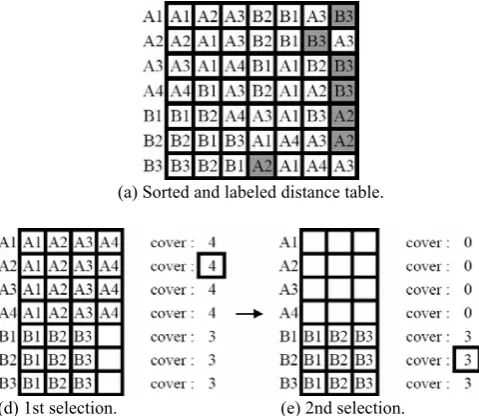
Initially, if only A2 and B3 are selected as a prototype set and used as a boundary instead of NUN, as shown in Fig. 2 (a), the MCSI will obtain A2 and B3 as a prototype set. Hence, the optimality depends on how to initially label the boundary.

(a) Sorted and labeled distance table.

(d) 1st selection. (e) 2nd selection. Fig. 2 Illustration of another selection approach

IV. REINFORCEMENT LEARNING ALGORITHM FOR THE MCSI

PROBLEM

Reinforcement learning (RL) [4] is a framework consisting of the agent going through states and the environment. In each state, the agent learns which action to take by obtaining the reward from an environment. After taking an action, the agent receives a reward and moves on to the other state. The goal is to repeat taking action and learn the best action to take in order to obtain the largest total rewards (returns).

its action leads to the next state that is consistent (i.e. the state that represents a consistent prototype set) otherwise a reward of zero will be given. During an episode, the RL agent learns by averaging the expected returns of each action at each state and updating the state-action value function using a technique called Q-learning [4]. The agent can continue experiencing more episodes to learn more about a better way to deselect a prototype (thus gaining more returns).

The standard Q-learning algorithm is shown as follows: For each episode:

s = the start state with all prototypes While the episode does not end:

1) the agent selects an action a to deselect a prototype from the state s using policy derived from Q

2) the environment provides a reward for an action a

at the state s and generates the next state sn

3) the agent updates Q(s,a) using Watkin’s Q(λ) [4] 4) the agent goes to the next state sn(s=sn)

5) If the state s is the terminal state episode end = true;

The reward is set to favor a path that leads to the consistent state with the minimum number of prototypes. The environment gives a reward of zero for an action that leads to an inconsistent state. There are N prototypes in the start state. Any action that leads to the consistent next state will have a positive reward. The reward can be more than +1 if the previous action has a reward of zero.

The reward given for taking an action a from the state s

and advancing to the next state sn is defined as follows:

Reward(s, a, sn) = 0, if the state sn is not consistent

= P(scon) - P(sn), otherwise Where scon is the latest consistent state found in the current episode, and P(s) is the number of prototypes in the state s.

There are many ways to balance between exploration and exploitation. The popular method is the ε-greedy policy which is to choose an action that has maximum action value with probability 1 - ε + (ε / |A|) and choose all other actions with probability ε / |A| where A is a set of all possible actions at the current state. The other method is the softmax policy.

The softmax policy used in this paper is defined as follows:

With probability ε:

Select an action a randomly With probability 1 - ε:

Select an action a based on its action value with probability

(1 - ε) Q(s, a)1.4 / ∑Q(s, b)1.4

For all action b that has Q(s, b) > 0.

This policy is adjusted to suit the MCSI problem which has many actions to choose at each state.

Fig. 3 The sequences of moves made by the RL agent

Fig. 3 illustrates the sequences of moves that the agent made in 2 episodes. An example data set used in this figure is the same data set as shown in Fig. 1 which consists of 7 data from two classes (4 from class A and 3 from class B).

Initially, the value function Q(a) of each action is set to zero. In the first episode, the agent deselects A1, A2, B3, A4, B2, and B1 from the original set and the episode ends at the terminal state, represented by the double line rectangle, which has only A3 as a prototype in the set (thus cannot be made consistent by deselecting more prototypes). The best solution found in this episode is of size 4, {A3, A4, B1, B2} as represented by the thick line rectangle, thus the return of +3 is obtained and Q(a) is updated as shown in the figure.

In the next episode, the agent learns to exploit by deselecting A1, A2, and, B3 according to its Q(a) at its corresponding state, and incidentally deselects A4 from the state {A3, A4, B1, B2} in which the best action so far is not known, then tries to explore by deselecting B1 (as represented by the thick line) which ends up in a consistent state, {A3, B2}, and is given a reward of +2. In the end, the terminal state is the state {A3} and the best state in this episode is of size 2, the state {A3, B2}, which is the optimum solution, and the return of +5 is obtained. The inconsistent state is represented by the dashed line rectangle and the dashed lines from {A3, B1} to {B1} and from {A3, B2} to {B2} represent an unexplored path.

V. IMPROVING THE EFFECTIVENESS OF THE RLALGORITHM

ε-greedy policy if the agent fails to obtain the largest returns from that state. This hampers the agent’s effort to locate the better solution from many potential states.

For example, if the ε=0.1 is used in the ε-greedy policy, the agent will follow the path that leads to the smallest consistent state experienced so far for about 9 steps before the exploration step happens in the 10th step. If the exploration step at that state leads to an inconsistent state, the episode may end with no more rewards and fail to influence the change to the agent’s exploitation strategy. Consequently, the agent rarely returns to many consistent states located deeper than 10 steps unless they are part of the current best path.

To overcome this shortcoming, a simple modification to the algorithm is presented. The idea is to force the agent to return to the last known consistent state if the current path from that state is overly long or the agent moves to the dead end. This encourages the agent to try as many actions as possible from that consistent state. The agent will eventually reach the smaller consistent state if there is one. The smaller consistent state then becomes the last known consistent state. The maximum steps allowed in the episode must be defined otherwise the episode will never end. The detail of the modification is as described below.

The new state transition function is defined as follows: After the agent selects an action a

and the environment generates the next state sn as usual If sn is consistent:

The environment provides a reward and proceeds as usual

Else:

If sn cannot leads to the smaller consistent state or with probability x

sn = the last known consistent state in the episode Reward = -1

Else:

Proceeds as usual

This transition function prevents the agent from moving through a long sequence of inconsistent states and ending the episode prematurely without a chance to explore a better path. The reward -1 is given as a penalty to signal the agent that it is better to explore another path instead.

The probability x can be any value between [0, 1]. The zero value means no backward transition is made unless the agent cannot deselect more prototypes. The value of 1 means the agent always moves back to the last known consistent state within the episode if the move does not lead to the next consistent state with one less prototype. The value of 0.2 is selected here because it prevents a move through a very long sequence of inconsistent states, but still allows an agent to move through a sequence of states that has some intermediate inconsistent states (this case is as shown in Fig. 3) which may be longer than 2 steps.

The termination condition of the algorithm is also changed from reaching the terminal state (there are no terminal states here) to reaching the maximum steps allowed in each episode. The maximum steps can be any number larger than the size of the original data set, but 5 times of the size of the original data set is usually good.

It is clear that the agent’s behavior is not changed since the update rule for the state-action value function is still the same. The major change is in the state transition function which is defined by the environment.

The performance comparison of the standard RL and the modified RL for the MCSI problem is as shown in Fig. 4. Both algorithms use the ε-greedy policy. The data set used here is the IRIS data set of 150 data from 3 classes.

8 28 48 68 88 108 128 148

0 2000 4000 6000 8000 10000 12000 14000 16000 18000 20000

Steps

N

u

mb

er

o

f

P

ro

to

typ

es

Fig. 4 Performance comparison of the standard RL and the modified RL for the MCSI problem

Each point in the graph shows the best consistent state with the smallest number of prototypes found in each episode. The cross points show the results of the standard RL algorithm while the round points show the results of the modified RL algorithm. Each point in the graph is the size of the best consistent subset found in each episode associated with the cumulative steps used by the algorithm. The best state in the later episode keeps getting better but not monotonically depending on the exploration rate parameter (i.e. the ε). Each episode takes about 150 steps in the standard RL and about 750 steps in the modified RL. The size of the best solutions found by the modified RL algorithm in each episode vary from 10 to 18 prototypes while the standard RL gets stuck in the long sequence of inconsistent states in some episodes and the size of the best solutions vary from 14 to 147 prototypes. The modified RL algorithm finds the solution of size 14 at the first episode as it also learns within an episode. The optimum set of 10 prototypes [5], [7] is eventually found by the modified RL algorithm while the best that the standard RL algorithm can find is of size 14 in this case.

VI. EXPERIMENTAL RESULTS

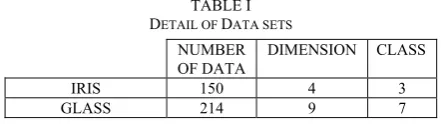
The size of the prototype set obtained from the standard RL algorithm is compared to the proposed modified RL algorithm and the standard MCSI [3] algorithm on the test data sets available at UCI site [6]. The test data sets are as shown in Table I.

TABLE I DETAIL OF DATA SETS

NUMBER OF DATA

DIMENSION CLASS

IRIS 150 4 3

GLASS 214 9 7

table II.

TABLE II

THE RESULTS OF THE ALGORITHMS FOR THE IRIS DATA SET

NUMBER OF PROTOTYPES

10 11 12 13 14 15 16 17

MCSI - - - - - 10 - -

Standard RL (ε-greedy)

- 1 - 2 2 2 2 1

Standard RL (softmax)

- 2 1 2 2 2 1 -

Modified RL (ε-greedy)

7 3 - - - -

Modified RL (softmax)

7 3 - - - -

In the IRIS data set case, the optimum set was found with size 10 [5], [7], the standard MCSI method’s [3] result is 15. The standard RL does not perform well (for both ε-greedy and softmax). It finds the result with the size smaller than 15 in some cases but performs poorer than the standard MCSI in the other cases. In addition, it could not find the optimum size (10 prototypes). The modified RL outperforms the standard RL and even finds the optimum size in most cases. It always performs better than the standard MCSI.

TABLE III

THE RESULTS OF THE ALGORITHMS FOR THE GLASS DATA SET

NUMBER OF PROTOTYPES

80 81 82 83 84 85

MCSI - - - 10

Modified RL (ε-greedy)

- - 1 3 6 -

Modified RL (softmax)

- 1 3 3 2 1

As shown in table III, the modified RL algorithm performs slightly better than the standard MCSI method in this data set. The softmax algorithm has more variance on the results obtained, but the best solution obtained by this method is better than the ε-greedy method in this case. The results from the standard RL are omitted here.

VII. CONCLUSION

This paper presents a reinforcement learning approach to the solution of the MCSI problem. The traditional RL method has some drawbacks and is easily being trapped in the local optimum. However, with a simple modification, the RL agent is able to get better results or obtain the optimum solution. Compared to the standard MCSI method, which is a greedy local search that usually obtains a suboptimum solution, the proposed method performs better as it learns to make a correct move through many trials in the potential region in the search space.

REFERENCES

[1] T. M. Cover and P. E. Hart, “Nearest Neighbor Pattern Classification”, IEEE Transactions on Information Theory, Vol. IT-13, No. 1, January 1967, pp. 21-27.

[2] P. E. Hart, “The Condensed Nearest Neighbor Rule”, IEEE Transactions on Information Theory, Vol. 14, 1968, pp. 515-516. [3] B. V. Dasarathy, “Minimal Consistent Set (MCS) Identification for

Optimal Nearest Neighbor Decision Systems Design”, IEEE Transactions on Systems, Man and Cybernetics, Vol. 24, No. 3, 1994, pp. 511-517.

[4] R. S. Sutton and A. G. Barto, “Reinforcement learning: An introduction.” MIT Press, Cambridge, MA, 1998.

[5] V. Cerveron and F. J. Ferri, “Another move toward the minimum consistent subset: a tabu search approach to the condensed nearest neighbor rule”, IEEE Transactions on Systems, Man and Cybernetics, Vol. 31, No. 3, 2001, pp. 408-413.

[6] Department of Information and Computer Science, University of California, Irvine. “UCI Machine Learning Repository” [Online]. Available: http://www.ics.uci.edu/~mlearn/MLRepository.html. 1998. [7] K. Kangkan, B. Kruatrachue, “Minimal Consistent Subset Selection as