A Generative Word Embedding Model and its Low Rank Positive
Semidefinite Solution
Shaohua Li1, Jun Zhu2, Chunyan Miao1
1Joint NTU-UBC Research Centre of Excellence in Active Living for the Elderly (LILY),
Nanyang Technological University, Singapore
2Tsinghua University, P.R. China
[email protected], [email protected], [email protected]
Abstract
Most existing word embedding methods can be categorized into Neural Embedding Models and Matrix Factorization (MF)-based methods. However some mod-els are opaque to probabilistic interpre-tation, and MF-based methods, typically solved using Singular Value Decomposi-tion (SVD), may incur loss of corpus in-formation. In addition, it is desirable to incorporate global latent factors, such as topics, sentiments or writing styles, into the word embedding model. Since gen-erative models provide a principled way to incorporate latent factors, we propose a generative word embedding model, which is easy to interpret, and can serve as a basis of more sophisticated latent factor models. The model inference reduces to a low rank weighted positive semidefinite approximation problem. Its optimization is approached by eigendecomposition on a submatrix, followed by online blockwise regression, which is scalable and avoids the information loss in SVD. In experi-ments on 7 common benchmark datasets, our vectors are competitive to word2vec, and better than other MF-based methods. 1 Introduction
The task of word embedding is to model the distri-bution of a word and its context words using their corresponding vectors in a Euclidean space. Then by doing regression on the relevant statistics de-rived from a corpus, a set of vectors are recovered which best fit these statistics. These vectors, com-monly referred to as the embeddings, capture se-mantic/syntactic regularities between the words.
The core of a word embedding method is the
link functionthat connects the input — the embed-dings, with the output — certain corpus statistics.
Based on the link function, the objective function is developed. The reasonableness of the link func-tion impacts the quality of the obtained embed-dings, and different link functions are amenable to different optimization algorithms, with different scalability. Based on the forms of the link func-tion and the optimizafunc-tion techniques, most meth-ods can be divided into two classes: the traditional
neural embedding models, and more recent low rank matrix factorization methods.
The neural embedding models use thesoftmax link function to model the conditional distribution of a word given its context (or vice versa) as a function of the embeddings. The normalizer in the softmax function brings intricacy to the optimiza-tion, which is usually tackled by gradient-based methods. The pioneering work was (Bengio et al., 2003). Later Mnih and Hinton (2007) propose three different link functions. However there are interaction matrices between the embeddings in all these models, which complicate and slow down the training, hindering them from being trained on huge corpora. Mikolov et al. (2013a) and Mikolov et al. (2013b) greatly simplify the condi-tional distribution, where the two embeddings in-teract directly. They implemented the well-known “word2vec”, which can be trained efficiently on huge corpora. The obtained embeddings show ex-cellent performance on various tasks.
Low-Rank Matrix Factorization (MF in short) methods include various link functions and opti-mization methods. The link functions are usu-ally not softmax functions. MF methods aim to reconstruct certain corpus statistics matrix by the product of two low rank factor matrices. The ob-jective is usually to minimize the reconstruction error, optionally with other constraints. In this line of research, Levy and Goldberg (2014b) find that “word2vec” is essentially doing stochastic weighted factorization of the word-context point-wise mutual information (PMI) matrix. They then
factorize this matrix directly as a new method. Pennington et al. (2014) propose a bilinear regres-sion function of the conditional distribution, from which a weighted MF problem on the bigram log-frequency matrix is formulated. Gradient Descent is used to find the embeddings. Recently, based on the intuition that words can be organized in se-mantic hierarchies, Yogatama et al. (2015) add hi-erarchical sparse regularizers to the matrix recon-struction error. With similar techniques, Faruqui et al. (2015) reconstruct a set of pretrained embed-dings using sparse vectors of greater dimensional-ity. Dhillon et al. (2015) apply Canonical Corre-lation Analysis (CCA) to the word matrix and the context matrix, and use the canonical correlation vectors between the two matrices as word embed-dings. Stratos et al. (2014) and Stratos et al. (2015) assume a Brown language model, and prove that doing CCA on the bigram occurrences is equiva-lent to finding a transformed solution of the lan-guage model. Arora et al. (2015) assume there is a hidden discourse vector on a random walk, which determines the distribution of the current word. The slowly evolving discourse vector puts a con-straint on the embeddings in a small text window. The maximum likelihood estimate of the embed-dings within this text window approximately re-duces to a squared norm objective.
There are two limitations in current word em-bedding methods. The first limitation is, all MF-based methods map words and their context words to two different sets of embeddings, and then em-ploy Singular Value Decomposition (SVD) to ob-tain a low rank approximation of the word-context matrixM. As SVD factorizes M>M, some in-formation in M is lost, and the learned embed-dings may not capture the most significant regu-larities inM. Appendix A gives a toy example on which SVD does not work properly.
The second limitation is, a generative model for documents parametered by embeddings is absent in recent development. Although (Stratos et al., 2014; Stratos et al., 2015; Arora et al., 2015) are based on generative processes, the generative pro-cesses are only for deriving the local relationship between embeddings within a small text window, leaving the likelihood of a document undefined. In addition, the learning objectives of some mod-els, e.g. (Mikolov et al., 2013b, Eq.1), even have no clear probabilistic interpretation. A genera-tive word embedding model for documents is not
only easier to interpret and analyze, but more im-portantly, provides a basis upon which document-levelgloballatent factors, such as document topics (Wallach, 2006), sentiments (Lin and He, 2009), writing styles (Zhao et al., 2011b), can be incor-porated in a principled manner, to better model the text distribution and extract relevant information.
Based on the above considerations, we pro-pose to unify the embeddings of words and con-text words. Our link function factorizes into three parts: the interaction of two embeddings capturing linear correlations of two words, a residual captur-ing nonlinear or noisy correlations, and the uni-gram priors. To reduce overfitting, we put Gaus-sian priors on embeddings and residuals, and ap-ply Jelinek-Mercer Smoothing to bigrams. Fur-thermore, to model the probability of a sequence of words, we assume that the contributions of more than one context word approximately add up. Thereby a generative model of documents is con-structed, parameterized by embeddings and resid-uals. The learning objective is to maximize the corpus likelihood, which reduces to a weighted low-rank positive semidefinite (PSD) approxima-tion problem of the PMI matrix. A Block Co-ordinate Descent algorithm is adopted to find an approximate solution. This algorithm is based on Eigendecomposition, which avoids information loss in SVD, but brings challenges to scalability. We then exploit the sparsity of the weight matrix and implement an efficient online blockwise re-gression algorithm. On seven benchmark datasets covering similarity and analogy tasks, our method achieves competitive and stable performance.
The source code of this method is provided at
https://github.com/askerlee/topicvec.
2 Notations and Definitions
Throughout the paper, we always use a uppercase bold letter asS,V to denote a matrix or set, a low-ercase bold letter asvwito denote a vector, a
nor-mal uppercase letter as N, W to denote a scalar constant, and a normal lowercase letter assi, wito denote a scalar variable.
Suppose a vocabularyS = {s1,· · · , sW}
con-sists of all the words, where W is the vocab-ulary size. We further suppose s1,· · · , sW are sorted in decending order of the frequency, i.e.
s1 is most frequent, and sW is least frequent. A document di is a sequence of words di =
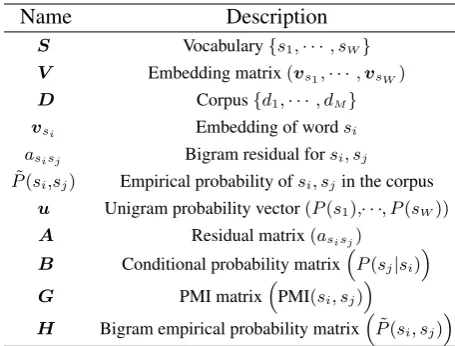
collec-Name Description
S Vocabulary{s1,· · ·, sW} V Embedding matrix(vs1,· · ·,vsW) D Corpus{d1,· · ·, dM} vsi Embedding of wordsi
asisj Bigram residual forsi, sj ˜
P(si,sj) Empirical probability ofsi, sjin the corpus u Unigram probability vector(P(s1),· · ·, P(sW)) A Residual matrix(asisj)
B Conditional probability matrixP(sj|si) G PMI matrixPMI(si, sj)
[image:3.595.70.298.61.234.2]
H Bigram empirical probability matrixP˜(si, sj)
Table 1: Notation Table
tion ofM documentsD ={d1,· · · , dM}. In the
vocabulary, each wordsiis mapped to a vectorvsi
inN-dimensional Euclidean space.
In a document, a sequence of words is referred to as a text window, denoted by wi,· · ·, wi+l, or
wi:wi+l in shorthand. A text window of chosen size cbefore a wordwi defines thecontext ofwi aswi−c,· · ·, wi−1. Here wi is referred to as the
focus word. Each context wordwi−jand the focus wordwicomprise a bigramwi−j, wi.
ThePointwise Mutual Informationbetween two wordssi, sjis defined as
PMI(si, sj) = logPP(s(si, sj) i)P(sj).
3 Link Function of Text
In this section, we formulate the probability of a sequence of words as a function of their embed-dings. We start from the link function of bigrams, which is the building blocks of a long sequence. Then this link function is extended to a text win-dow withccontext words, as a first-order approx-imation of the actual probability.
3.1 Link Function of Bigrams
We generalize the link function of “word2vec” and “GloVe” to the following:
P(si, sj) = exp
n
v>
sjvsi+asisj o
P(si)P(sj) (1)
The rationale for (1) originates from the idea of the Product of Experts in (Hinton, 2002). Sup-pose different types of semantic/syntactic regu-larities between si and sj are encoded in differ-ent dimensions of vsi,vsj. As exp{v>sjvsi} = Q
lexp{vsi,l·vsj,l}, this means the effects of
dif-ferent regularities on the probability are combined
by multiplying together. Ifsiandsj are indepen-dent, their joint probability should beP(si)P(sj). In the presence of correlations, the actual joint probabilityP(si, sj)would be a scaling of it. The scale factor reflects how muchsi andsj are pos-itively or negatively correlated. Within the scale factor,v>
sjvsi captures linear interactions between
si andsj, the residualasisj captures nonlinear or
noisy interactions. In applications, onlyv> sjvsi is
of interest. Hence the bigger magnitudev> sjvsi is
of relative toasisj, the better.
Note that we do not assume asisj = asjsi.
This provides the flexibilityP(si, sj)=6 P(sj, si), agreeing with the asymmetry of bigrams in natu-ral languages. At the same time,v>
sjvsiimposes a
symmetric part betweenP(si, sj)andP(sj, si). (1) is equivalent to
P(sj|si)=exp
n
v>
sjvsi+asisj+ logP(sj) o
, (2)
logPP(s(js|si)
j) =v >
sjvsi+asisj. (3)
(3) of all bigrams is represented in matrix form: V>V +A=G, (4) whereGis the PMI matrix.
3.1.1 Gaussian Priors on Embeddings
When (1) is employed on the regression of empir-ical bigram probabilities, a practempir-ical issue arises: more and more bigrams have zero frequency as the constituting words become less frequent. A zero-frequency bigram does not necessarily imply negative correlation between the two constituting words; it could simply result from missing data. But in this case, even after smoothing, (1) will forcev>
sjvsi +asisj to be a big negative number,
makingvsi overly long. The increased magnitude
of embeddings is a sign of overfitting.
To reduce overfitting of embeddings of infre-quent words, we assign a Spherical Gaussian prior
N(0, 1
2µiI)tovsi:
P(vsi)∼exp{−µikvsik2},
where the hyperparameterµi increases as the fre-quency ofsi decreases.
3.1.2 Gaussian Priors on Residuals We wish v>
sjvsi in (1) captures as much
corre-lations between si and sj as possible. Thus the smallerasisj is, the better. In addition, the more
To this end, we penalize the residual asisj
by f(˜P(si, sj))a2sisj, where f(·) is a
nonnega-tive monotonic transformation, referred to as the
weighting function. Lethij denoteP˜(si, sj), then the total penalty of all residuals are the square of theweighted Frobenius normofA:
X
si,sj∈S
f(hij)a2sisj =kAk2f(H). (5)
By referring to “GloVe”, we use the following weighting function, and find it performs well:
f(hij) =
√
hij
Ccut p
hij < Ccut, i6=j
1 phij ≥Ccut, i6=j
0 i=j
,
where Ccut is chosen to cut the most frequent
0.02%of the bigrams off at1. Whensi =sj, two identical words usually have much smaller proba-bility to collocate. HenceP˜(si, si)does not reflect the true correlation of a word to itself, and should not put constraints to the embeddings. We elimi-nate their effects by settingf(hii)to0.
If the domain ofAis the whole spaceRW×W, then this penalty is equivalent to a Gaussian prior
N 0,2f(1hij)on eachasisj. The variances of the
Gaussians are determined by the bigram empirical probability matrixH.
3.1.3 Jelinek-Mercer Smoothing of Bigrams As another measure to reduce the impact of miss-ing data, we apply the commonly used Jelinek-Mercer Smoothing (Zhai and Lafferty, 2004) to smooth the empirical conditional probability
˜
P(sj|si)by the unigram probabilityP˜(sj)as:
˜
Psmoothed(sj|si) = (1−κ) ˜P(sj|si)+κP(sj). (6) Accordingly, the smoothed bigram empirical joint probability is defined as
˜
P(si, sj) = (1−κ) ˜P(si, sj)+κP(si)P(sj). (7) In practice, we find κ = 0.02 yields good re-sults. Whenκ ≥ 0.04, the obtained embeddings begin to degrade withκ, indicating that smoothing distorts the true bigram distributions.
3.2 Link Function of a Text Window
In the previous subsection, a regression link func-tion of bigram probabilities is established. In this section, we adopt a first-order approximation based on Information Theory, and extend the link function to a longer sequencew0,· · ·, wc−1, wc.
Decomposing a distribution conditioned on n
random variables as the conditional distributions
on its subsets roots deeply in Information The-ory. This is an intricate problem because there could be both (pointwise) redundant information
and (pointwise)synergistic informationamong the conditioning variables (Williams and Beer, 2010). They are both functions of the PMI. Based on an analysis of the complementing roles of these two types of pointwise information, we assume they are approximately equal and cancel each other when computing the pointwise interaction infor-mation. See Appendix B for a detailed discussion. Following the above assumption, we have PMI(w2;w0, w1)≈PMI(w2;w0)+PMI(w2;w1):
logP(w0, w1|w2)
P(w0, w1) ≈log
P(w0|w2)
P(w0) +log
P(w1|w2)
P(w1) . Plugging (1) and (3) into the above, we obtain
P(w0, w1, w2)
≈exp
X2
i,j=0
i6=j
(v>
wivwj +awiwj) + 2 X
i=0
logP(wi)
.
We extend the above assumption to that the pointwise interaction information is still close to
0 within a longer text window. Accordingly the above equation extends to a context of sizec >2:
P(w0,· · ·, wc)
≈exp
Xc
i,j=0
i6=j
(v>
wivwj +awiwj) +
c
X
i=0
logP(wi)
.
From it derives the conditional distribution of
wc, given its contextw0,· · ·, wc−1:
P(wc|w0 :wc−1)=PP(w(w0,· · ·, wc) 0,· · ·, wc−1)
≈P(wc) exp
v> wc
c−1 X
i=0
vwi+
c−1 X
i=0
awiwc
. (8)
4 Generative Process and Likelihood We proceed to assume the text is generated from a
Markov chainof orderc, i.e., a word only depends on words within its context of size c. Given the hyperparameterµ= (µ1,· · ·, µW), the generative
process of the whole corpus is:
1. For each word si, draw the embedding vsi
from N(0,21µiI);
2. For each bigram si, sj, draw the residual
asisjfrom N
0, 1 2f(hij)
;
3. For each document di, for the j-th word, draw word wij from S with probability
vw0 vw1 · · · vwc
d
V A
µi
vsi
hij
[image:5.595.91.266.59.229.2]aij
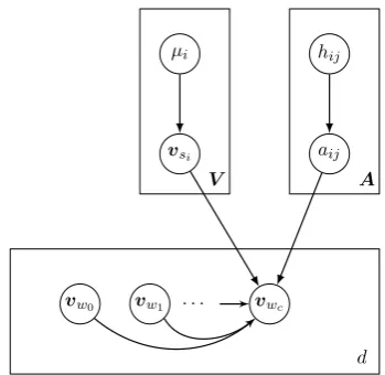
Figure 1: The Graphical Model of PSDVec
The above generative process for a documentdis presented as a graphical model in Figure 1.
Based on this generative process, the probabil-ity of a document di can be derived as follows, given the embeddings and residualsV,A:
P(di|V,A)
=
Li Y
j=1
P(wij) exp
v> wij
j−1 X
k=j−c vwik+
j−1 X
k=j−c
awikwij
.
The complete-data likelihood of the corpus is:
p(D,V,A)
=
W
Y
i=1
N(0,2Iµ
i) W,WY
i,j=1 N
0,2f(1h
ij)
YM
i=1
p(di|V,A)
=Z(H1,µ)expn−
W,WX
i,j=1
f(hi,j)a2sisj−
W
X
i=1
µikvsik2
o
·
M,LYi
i,j=1
P(wij) exp
v> wij
j−1 X
k=j−c vwik+
j−1 X
k=j−c
awikwij
,
whereZ(H,µ)is the normalizing constant. Taking the logarithm of both sides of
p(D,A,V)yields
logp(D,V,A)
=C0−logZ(H,µ)− kAk2f(H)−
W
X
i=1
µikvsik2
+
M,LXi
i,j=1
v> wij
j−1 X
k=j−c vwik+
j−1 X
k=j−c
awikwij
, (9)
whereC0=PM,Li,j=1ilogP(wij)is constant.
5 Learning Algorithm 5.1 Learning Objective
The learning objective is to find the embeddings V that maximize the corpus log-likelihood (9).
Letxij denote the (smoothed) frequency of bi-gramsi, sj in the corpus. Then (9) is sorted as:
logp(D,V,A)
=C0−logZ(H,µ)− kAk2f(H)−
W
X
i=1
µikvsik2
+
W,WX
i,j=1
xij(v>sivsj+asisj). (10)
As the corpus size increases,
PW,W
i,j=1xij(v>sivsj+asisj) will dominate the
parameter prior terms. Then we can ignore the prior terms when maximizing (10).
maxXxij(v>sivsj+asisj)
=Xxij
·maxXP˜smoothed(si, sj) logP(si, sj). As both {P˜smoothed(si, sj)} and {P(si, sj)} sum to 1, the above sum is maximized when
P(si, sj) = ˜Psmoothed(si, sj).
The maximum likelihood estimator is then:
P(sj|si) = ˜Psmoothed(sj|si),
v>
sivsj +asisj = log
˜
Psmoothed(sj|si)
P(sj) . (11)
Writing (11) in matrix form: B∗ =P˜
smoothed(sj|si)
si,sj∈S
G∗ = logB∗−logu⊗(1· · ·1), (12)
where “⊗” is the outer product. Now we fix the values ofv>
sivsj +asisj at the
above optimal. The corpus likelihood becomes
logp(D,V,A) =C1− kAk2f(H)−
W
X
i=1
µikvsik2,
subject to V>V +A=G∗, (13) where C1 = C0 +Pxijlog ˜Psmoothed(si, sj) −
logZ(H,µ)is constant.
5.2 LearningV as Low Rank PSD Approximation
Algorithm 1BCD algorithm for finding a unreg-ularized rank-N weighted PSD approximant. Input: matrixG∗, weight matrixW =f(H),
iteration numberT, rankN
Randomly initializeX(0)
fort= 1,· · ·,T do
Gt=W ◦G∗+ (1−W)◦X(t−1) X(t)=PSD Approximate(G
t, N) end for
λ,Q= Eigen Decomposition(X(T))
V∗= diag(λ1
2[1:N])·Q>[1:N] Output:V∗
arg max
V logp(D,V,A)
= arg min
V kG
∗−V>Vk f(H)+
W
X
i=1
µikvsik2. (14)
LetX = V>V. ThenX is positive semidef-inite of rank N. Finding V that minimizes (14) is equivalent to finding a rank-N weighted posi-tive semidefinite approximantXofG∗, subject to Tikhonov regularization. This problem does not admit an analytic solution, and can only be solved using local optimization methods.
First we consider a simpler case where all the words in the vocabulary are enough frequent, and thus Tikhonov regularization is unnecessary. In this case, we set∀µi = 0, and (14) becomes an unregularized optimization problem. We adopt the Block Coordinate Descent (BCD) algorithm1 in
(Srebro et al., 2003) to approach this problem. The original algorithm is to find a generic rank-N ma-trix for a weighted approximation problem, and we tailor it by constraining the matrix within the positive semidefinite manifold.
We summarize our learning algorithm in Al-gorithm 1. Here “◦” is the entry-wise prod-uct. We suppose the eigenvalues λ returned by Eigen Decomposition(X) are in descending or-der.Q>[1:N]extracts the 1 toN rows fromQ>.
One key issue is how to initializeX. Srebro et al. (2003) suggest to setX(0)=G∗, and point out
that X(0)=0 is far from a local optimum, thus requires more iterations. However we find G∗ is
also far from a local optimum, and this setting con-verges slowly too. SettingX(0) =G∗/2usually
1It is referred to as an Expectation-Maximization algo-rithm by the original authors, but we think this is a misnomer.
yields a satisfactory solution in a few iterations. The subroutine PSD Approximate() computes the unweighted nearest rank-N PSD approxima-tion, measured in F-norm (Higham, 1988).
5.3 Online Blockwise Regression ofV
In Algorithm 1, the essential subroutine PSD Approximate() does eigendecomposi-tion on Gt, which is dense due to the logarithm transformation. Eigendecomposition on aW×W
dense matrix requiresO(W2) space andO(W3)
time, difficult to scale up to a large vocabulary. In addition, the majority of words in the vocabulary are infrequent, and Tikhonov regularization is necessary for them.
It is observed that, as words become less fre-quent, fewer and fewer words appear around them to form bigrams. Remind that the vocabulary S = {s1,· · · , sW} are sorted in decending or-der of the frequency, hence the lower-right blocks ofH andf(H) are very sparse, and cause these blocks in (14) to contribute much less penalty rela-tive to other regions. Therefore these blocks could be ignored when doing regression, without sacri-ficing too much accuracy. This intuition leads to the followingonline blockwise regression.
The basic idea is to select a small set (e.g. 30,000) of the most frequent words as the core words, and partition the remainingnoncore words
into sets of moderate sizes. Bigrams consist-ing of two core words are referred to ascore bi-grams, which correspond to the top-left blocks of G and f(H). The embeddings of core words are learned approximately using Algorithm 1, on the top-left blocks of Gandf(H). Then we fix the embeddings of core words, and find the em-beddings of each set of noncore words in turn. After ignoring the lower-right regions of G and
f(H) which correspond to bigrams of two non-core words, thequadratic termsof noncore em-beddings are ignored. Consequently, finding these embeddings becomes aweighted ridge regression
problem, which can be solved efficiently in closed-form. Finally we combine all embeddings to get the embeddings of the whole vocabulary. The de-tails are as follows:
1. Partition S into K consecutive groups S1,· · · ,Sk. Take K = 3 as an example. The first group is core words;
in this example as
GG1121 GG1222 GG1323
G31 G32 G33 .
Partition f(H),A in the same way. G11, f(H)11,A11 correspond to core
bi-grams. PartitionV into |{z} S1 V1
| {z } S2 V2
| {z } S3 V3
;
3. SolveV>
1V1+A11=G11using Algorithm
1, and obtain core embeddingsV∗
1;
4. SetV1 = V∗1, and findV∗2 that minimizes
the total penalty of the12-th and 21-th blocks of residuals (the 22-th block is ignored due to its high sparsity):
arg min
V2 kG12−V
>
1V2k2f(H)12
+kG21−V>2V1k2f(H)21+ X
si∈S2
µikvsik2
= arg min
V2 kG12−V
>
1V2k2f¯(H)12+
X
si∈S2
µikvsik2,
where f¯(H)12 = f(H)12 + f(H)>21;
G12 =
G12 ◦f(H)12+G>21◦f(H)>21
/f(H)12+f(H)>21
is the weighted aver-age ofG12andG>21, “◦” and “/” are
element-wise product and division, respectively. The columns inV2are independent, thus for each
vsi, it is a separate weighted ridge regression
problem, whose solution is (Holland, 1973): v∗
si=(V>1diag(f¯i)V1+µiI)−1V>1diag(f¯i)¯gi,
wheref¯i andg¯i are columns corresponding tosiinf¯(H)12 andG12, respectively;
5. For any other set of noncore words Sk, find V∗
kthat minimizes the total penalty of the1k -th andk1-th blocks, ignoring all other kj-th andjk-th blocks;
6. Combine all subsets of embeddings to form V∗. HereV∗ = (V∗
1,V∗2,V∗3).
6 Experimental Results
We trained our model along with a few state-of-the-art competitors on Wikipedia, and evaluated the embeddings on 7 common benchmark sets. 6.1 Experimental Setup
Our own method is referred to asPSD. The com-petitors include:
• (Mikolov et al., 2013b): word2vec2, or
SGNS in some literature;
2https://code.google.com/p/word2vec/
• (Levy and Goldberg, 2014b): thePPMI ma-trix without dimension reduction, and SVD of PPMI matrix, both yielded by hyperwords;
• (Pennington et al., 2014):GloVe3;
• (Stratos et al., 2015):Singular4, which does
SVD-based CCA on the weighted bigram fre-quency matrix;
• (Faruqui et al., 2015):Sparse5, which learns
new sparse embeddings in a higher dimen-sional space from pretrained embeddings. All models were trained on the English Wikipedia snapshot in March 2015. After removing non-textual elements and non-English words, 2.04 bil-lion words were left. We used the default hyperpa-rameters in Hyperwords when training PPMI and SVD. Word2vec, GloVe and Singular were trained with their own default hyperparameters.
The embedding sets Reg-180K and PSD-Unreg-180K were trained using our online block-wise regression. Both sets contain the embed-dings of the most frequent 180,000 words, based on 25,000 core words. PSD-Unreg-180K was traind with all µi = 0, i.e. disabling Tikhonov regularization. PSD-Reg-180K was trained with
µi =
2 i∈[25001,80000] 4 i∈[80001,130000] 8 i∈[130001,180000]
,i.e. increased
regularization as the sparsity increases. To con-trast with the batch learning performance, the per-formance of PSD-25K is listed, which contains the core embeddings only. PSD-25K took advantages that it contains much less false candidate words, and some test tuples (generally harder ones) were not evaluated due to missing words, thus its scores are not comparable to others.
Sparse was trained with PSD-180K-reg as the input embeddings, with default hyperparameters.
The benchmark sets are almost identical to those in (Levy et al., 2015), except that (Luong et al., 2013)’s Rare Words is not included, as many rare words are cut off at the frequency 100, mak-ing more than 1/3 of test pairs invalid.
Word Similarity There are 5 datasets: Word-Sim Word-Similarity (WS Sim) and WordSim Related-ness (WS Rel) (Zesch et al., 2008; Agirre et al., 2009), partitioned from WordSim353 (Finkelstein et al., 2002); Bruni et al. (2012)’s MENdataset;
Similarity Tasks Analogy Tasks
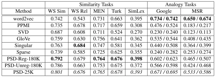
Method WS Sim WS Rel MEN Turk SimLex Google MSR
[image:8.595.73.525.60.221.2]word2vec 0.742 0.543 0.731 0.663 0.395 0.734/0.742 0.650/0.674 PPMI 0.735 0.678 0.717 0.659 0.308 0.476 / 0.524 0.183 / 0.217 SVD 0.687 0.608 0.711 0.524 0.270 0.230 / 0.240 0.123 / 0.113 GloVe 0.759 0.630 0.756 0.641 0.362 0.535 / 0.544 0.408 / 0.435 Singular 0.763 0.684 0.747 0.581 0.345 0.440 / 0.508 0.364 / 0.399 Sparse 0.739 0.585 0.725 0.625 0.355 0.240 / 0.282 0.253 / 0.274 PSD-Reg-180K 0.792 0.679 0.764 0.676 0.398 0.602 / 0.623 0.465 / 0.507 PSD-Unreg-180K 0.786 0.663 0.753 0.675 0.372 0.566 / 0.598 0.424 / 0.468 PSD-25K 0.801 0.676 0.765 0.678 0.393 0.671 / 0.695 0.533 / 0.586
Table 2: Performance of each method across different tasks.
Radinsky et al. (2011)’s MechanicalTurkdataset; and (Hill et al., 2014)’sSimLex-999 dataset. The embeddings were evaluated by the Spearman’s rank correlation with the human ratings.
Word Analogy The two datasets are MSR’s analogy dataset (Mikolov et al., 2013c), with 8000 questions, andGoogle’s analogy dataset (Mikolov et al., 2013a), with 19544 questions. After filtering questions involving out-of-vocabulary words, i.e. words that appear less than 100 times in the cor-pus, 7054 instances in MSR and 19364 instances in Google were left. The analogy questions were answered using 3CosAdd as well as 3CosMul pro-posed by Levy and Goldberg (2014a).
6.2 Results
Table 2 shows the results on all tasks. Word2vec significantly outperformed other methods on anal-ogy tasks. PPMI and SVD performed much worse on analogy tasks than reported in (Levy et al., 2015), probably due to sub-optimal hyperparam-eters. This suggests their performance is unstable. The new embeddings yielded by Sparse systemat-icallydegradedcompared to the old embeddings, contradicting the claim in (Faruqui et al., 2015).
Our method PSD-Reg-180K performed well consistently, and is best in 4 similarity tasks. It performed worse than word2vec on analogy tasks, but still better than other MF-based meth-ods. By comparing to PSD-Unreg-180K, we see Tikhonov regularization brings 1-4% performance boost across tasks. In addition, on similarity tasks, online blockwise regression only degrades slightly compared to batch factorization. Their perfor-mance gaps on analogy tasks were wider, but this might be explained by the fact that some hard cases were not counted in PSD-25K’s evaluation,
due to its limited vocabulary.
7 Conclusions and Future Work
In this paper, inspired by the link functions in previous works, with the support from Informa-tion Theory, we propose a new link funcInforma-tion of a text window, parameterized by the embeddings of words and the residuals of bigrams. Based on the link function, we establish a generative model of documents. The learning objective is to find a set of embeddings maximizing their posterior likeli-hood given the corpus. This objective is reduced to weighted low-rank positive-semidefinite approxi-mation, subject to Tikhonov regularization. Then we adopt a Block Coordinate Descent algorithm, jointly with an online blockwise regression algo-rithm to find an approximate solution. On seven benchmark sets, the learned embeddings show competitive and stable performance.
In the future work, we will incorporate global latent factors into this generative model, such as topics, sentiments, or writing styles, and develop more elaborate models of documents. Through learning such latent factors, important summary information of documents would be acquired, which are useful in various applications.
Acknowledgments
Appendix A Possible Trap in SVD
SupposeM is the bigram matrix of interest. SVD embeddings are derived from the low rank approx-imation ofM>M, by keeping the largest singular values/vectors. When some of these singular val-ues correspond to negative eigenvalval-ues, undesir-able correlations might be captured. The follow-ing is an example of approximatfollow-ing a PMI matrix. A vocabulary consists of 3 words s1, s2, s3.
Two corpora derive two PMI matrices: M(1) =10..4 08 2..8 06 0
0 0 2
, M(2)=−01.2.6−−21..6 02 0
0 0 2
.
They have identical left singular matrix and sin-gular values (3,2,1), but their eigenvalues are
(3,2,1)and(−3,2,1), respectively.
In a rank-2 approximation, the largest two singular values/vectors are kept, and M(1) and
M(2) yield identical SVD embeddings V =
(0.45 0.89 0
0 0 1)(the rows may be scaled depending on
the algorithm, without affecting the validity of the following conclusion). The embeddings ofs1 and
s2 (columns 1 and 2 of V) point at the same
di-rection, suggesting they are positively correlated. However asM(2)1,2 =M(2)2,1 =−1.6 <0, they are actually negatively correlated in the second cor-pus. This inconsistency is because the principal eigenvalue ofM(2)is negative, and yet the
corre-sponding singular value/vector is kept.
When using eigendecomposition, the largest two positive eigenvalues/eigenvectors are kept. M(1) yields the same embeddings V. M(2) yieldsV(2) = −0.89 0.45 0
0 0 1.41
, which correctly preserves the negative correlation betweens1, s2.
Appendix B Information Theory
Redundant information refers to the reduced un-certainty by knowing the value of any one of the conditioning variables (hence redundant). Syner-gistic information is the reduced uncertainty as-cribed to knowing all the values of conditioning variables, that cannot be reduced by knowing the value of any variable alone (hence synergistic).
The mutual informationI(y;xi)and the redun-dant information Rdn(y;x1, x2)are defined as:
I(y;xi) =EP(xi,y)[log
P(y|xi)
P(y) ]
Rdn(y;x1, x2) =EP(y)
min
x1,x2EP(xi|y)[log
P(y|xi)
P(y) ]
The synergistic information Syn(y;x1, x2) is
defined as the PI-function in (Williams and Beer, 2010), skipped here.
I(y;x1) I(y;x2) Syn(y;x1,x2)
I(y;x1,x2)
[image:9.595.345.485.63.169.2]Rdn(y;x1,x2)
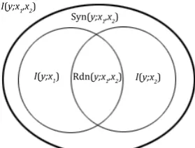
Figure 2: Different types of information among 3 random variables y, x1, x2. I(y;x1, x2) is
the mutual information between y and (x1, x2).
Rdn(y;x1, x2) and Syn(y;x1, x2) are the
redun-dant information and synergistic information be-tweenx1, x2, conditioningy, respectively.
The interaction information Int(x1, x2, y)
mea-sures the relative strength of Rdn(y;x1, x2) and
Syn(y;x1, x2)(Timme et al., 2014):
Int(x1, x2, y)
=Syn(y;x1, x2)−Rdn(y;x1, x2)
=I(y;x1, x2)−I(y;x1)−I(y;x2)
=EP(x1,x2,y)[log
P(x1)P(x2)P(y)P(x1, x2, y)
P(x1, x2)P(x1, y)P(x2, y) ]
Figure 2 shows the relationship of different information among 3 random variables y, x1, x2
(based on Fig.1 in (Williams and Beer, 2010)). PMI is the pointwise counterpart of mutual information I. Similarly, all the above concepts have their pointwise counterparts, obtained by dropping the expectation operator. Specifically, thepointwise interaction informationis defined as PInt(x1, x2, y) =PMI(y;x1, x2)−PMI(y;x1)−
PMI(y;x2) = logPP(x(1x)1P,x(x2)2P)P(x(1y,y)P)P(x(1x,x2,y2,y)).
If we know PInt(x1, x2, y), we can recover
PMI(y;x1, x2) from the mutual information over
the variable subsets, and then recover the joint distributionP(x1, x2, y).
As the pointwise redundant information PRdn(y;x1, x2) and the pointwise synergistic
information PSyn(y;x1, x2) are both
higher-order interaction terms, their magnitudes are usually much smaller than the PMI terms. We assume they are approximately equal, and thus cancel each other when computing PInt. Given this, PInt is always 0. In the case of three wordsw0, w1, w2, PInt(w0, w1, w2) = 0 leads to
References
Eneko Agirre, Enrique Alfonseca, Keith Hall, Jana Kravalova, Marius Pas¸ca, and Aitor Soroa. 2009. A study on similarity and relatedness using
distribu-tional and wordnet-based approaches. In
Proceed-ings of Human Language Technologies: The 2009 Annual Conference of the North American Chap-ter of the Association for Computational Linguistics, pages 19–27. Association for Computational Lin-guistics.
Sanjeev Arora, Yuanzhi Li, Yingyu Liang, Tengyu Ma, and Andrej Risteski. 2015. Random walks on discourse spaces: a new generative language model with applications to semantic word
embed-dings. ArXiv e-prints, arXiv:1502.03520 [cs.LG].
Yoshua Bengio, R´ejean Ducharme, Pascal Vincent, and Christian Jauvin. 2003. A neural probabilistic
lan-guage model. Journal of Machine Learning
Re-search, pages 1137–1155.
David M Blei, Andrew Y Ng, and Michael I Jordan.
2003. Latent dirichlet allocation. The Journal of
Machine Learning Research, 3:993–1022.
Elia Bruni, Gemma Boleda, Marco Baroni, and Nam-Khanh Tran. 2012. Distributional semantics in
tech-nicolor. In Proceedings of the 50th Annual
Meet-ing of the Association for Computational LMeet-inguis- Linguis-tics: Long Papers-Volume 1, pages 136–145. Asso-ciation for Computational Linguistics.
Scott C. Deerwester, Susan T Dumais, and Richard A. Harshman. 1990. Indexing by latent semantic
anal-ysis. J. Am. Soc. Inf. Sci.
Paramveer Dhillon, Dean P Foster, and Lyle H Ungar. 2011. Multi-view learning of word embeddings via
cca. InProceedings of Advances in Neural
Informa-tion Processing Systems, pages 199–207.
Paramveer S Dhillon, Dean P Foster, and Lyle H Ungar.
2015. Eigenwords: Spectral word embeddings. The
Journal of Machine Learning Research.
Manaal Faruqui, Yulia Tsvetkov, Dani Yogatama, Chris Dyer, and Noah A. Smith. 2015. Sparse
overcom-plete word vector representations. InProceedings of
ACL 2015.
Lev Finkelstein, Evgeniy Gabrilovich, Yossi Matias, Ehud Rivlin, Zach Solan, Gadi Wolfman, and Ey-tan Ruppin. 2002. Placing search in context: The
concept revisited. ACM Trans. Inf. Syst., 20(1):116–
131, January.
Amir Globerson, Gal Chechik, Fernando Pereira, and Naftali Tishby. 2007. Euclidean embedding of
co-occurrence data. Journal of Machine Learning
Re-search, vol. 8 (2007):2265–2295, Oct.
Nicholas J. Higham. 1988. Computing a nearest
sym-metric positive semidefinite matrix. Linear Algebra
and its Applications, 103(0):103 – 118.
Felix Hill, Roi Reichart, and Anna Korhonen. 2014. Simlex-999: Evaluating semantic models with
(gen-uine) similarity estimation. CoRR, abs/1408.3456.
Geoffrey Hinton. 2002. Training products of experts
by minimizing contrastive divergence.Neural
Com-putation, 14(8):1771–1800.
Paul W. Holland. 1973. Weighted Ridge Regression: Combining Ridge and Robust Regression Methods. NBER Working Papers 0011, National Bureau of Economic Research, Inc, September.
Daniel Hsu, Sham M Kakade, and Tong Zhang. 2012. A spectral algorithm for learning hidden markov
models. Journal of Computer and System Sciences,
78(5):1460–1480.
Omer Levy and Yoav Goldberg. 2014a. Linguistic reg-ularities in sparse and explicit word representations. InProceedings of CoNLL-2014, page 171.
Omer Levy and Yoav Goldberg. 2014b. Neural word
embeddings as implicit matrix factorization. In
Pro-ceedings of NIPS 2014.
Omer Levy, Yoav Goldberg, and Ido Dagan. 2015. Im-proving distributional similarity with lessons learned
from word embeddings. Transactions of the
Associ-ation for ComputAssoci-ational Linguistics, 3:211–225. Chenghua Lin and Yulan He. 2009. Joint
senti-ment/topic model for sentiment analysis. In
Pro-ceedings of the 18th ACM conference on Informa-tion and Knowledge Management, pages 375–384. ACM.
Minh-Thang Luong, Richard Socher, and Christo-pher D Manning. 2013. Better word representa-tions with recursive neural networks for morphol-ogy. CoNLL-2013, 104.
Thomas Mach. 2012. Eigenvalue Algorithms for
Sym-metric Hierarchical Matrices. Dissertation, Chem-nitz University of Technology.
Tomas Mikolov, Kai Chen, Greg Corrado, and Jeffrey Dean. 2013a. Efficient estimation of word
represen-tations in vector space. InProceedings of Workshop
at ICLR 2013.
Tomas Mikolov, Ilya Sutskever, Kai Chen, Greg S Cor-rado, and Jeff Dean. 2013b. Distributed representa-tions of words and phrases and their
compositional-ity. InProceedings of NIPS 2013, pages 3111–3119.
Tomas Mikolov, Wen-tau Yih, and Geoffrey Zweig. 2013c. Linguistic regularities in continuous space
word representations. In Proceedings of
HLT-NAACL 2013, pages 746–751.
Jeffrey Pennington, Richard Socher, and Christopher D
Manning. 2014. Glove: Global vectors for
word representation. Proceedings of the Empiricial
Methods in Natural Language Processing (EMNLP 2014), 12.
Kira Radinsky, Eugene Agichtein, Evgeniy
Gabrilovich, and Shaul Markovitch. 2011. A word at a time: Computing word relatedness using
temporal semantic analysis. In Proceedings of the
20th International Conference on World Wide Web, WWW ’11, pages 337–346, New York, NY, USA. ACM.
Nathan Srebro, Tommi Jaakkola, et al. 2003. Weighted
low-rank approximations. InProceedings of ICML
2003, volume 3, pages 720–727.
Karl Stratos, Do-kyum Kim, Michael Collins, and Daniel Hsu. 2014. A spectral algorithm for learn-ing class-based n-gram models of natural language. InProceedings of the Association for Uncertainty in Artificial Intelligence.
Karl Stratos, Michael Collins, and Daniel Hsu. 2015. Model-based word embeddings from
decomposi-tions of count matrices. In Proceedings of ACL
2015.
Mingkui Tan, Ivor W. Tsang, Li Wang, Bart Vander-eycken, and Sinno Jialin Pan. 2014. Riemannian
pursuit for big matrix recovery. In Proceedings of
ICML 2014, pages 1539–1547.
Nicholas Timme, Wesley Alford, Benjamin Flecker, and John M Beggs. 2014. Synergy, redundancy, and multivariate information measures: an
experi-mentalist’s perspective. Journal of Computational
Neuroscience, 36(2):119–140.
Hanna M Wallach. 2006. Topic modeling: beyond
bag-of-words. InProceedings of the 23rd
interna-tional conference on Machine learning, pages 977– 984. ACM.
Paul L Williams and Randall D Beer. 2010. Non-negative decomposition of multivariate information. arXiv preprint arXiv:1004.2515.
Yan Yan, Mingkui Tan, Ivor Tsang, Yi Yang, Chengqi Zhang, and Qinfeng Shi. 2015. Scalable maximum margin matrix factorization by active riemannian
subspace search. InProceedings of IJCAI 2015.
Dani Yogatama, Manaal Faruqui, Chris Dyer, and Noah A Smith. 2015. Learning word
representa-tions with hierarchical sparse coding. In
Proceed-ings of ICML 2015.
Torsten Zesch, Christof M¨uller, and Iryna Gurevych. 2008. Using wiktionary for computing semantic
re-latedness. InProceedings of AAAI 2008, volume 8,
pages 861–866.
Chengxiang Zhai and John Lafferty. 2004. A study of smoothing methods for language models applied to
information retrieval. ACM Transactions on
Infor-mation Systems (TOIS), 22(2):179–214.
Peilin Zhao, Steven CH Hoi, and Rong Jin. 2011a.
Double updating online learning. The Journal of
Machine Learning Research, 12:1587–1615. Wayne Xin Zhao, Jing Jiang, Jianshu Weng, Jing
He, Ee-Peng Lim, Hongfei Yan, and Xiaoming Li. 2011b. Comparing twitter and traditional
me-dia using topic models. In Advances in