Abstract— In this article, we are interested in the reactive behaviours navigation training of a mobile robot in an unknown environment. The method we will suggest ensures navigation in unknown environments with presence off different obstacles shape and consists in bringing the robot in a goal position, avoiding obstacles and releasing it from the tight corners and deadlock obstacles shape. This is difficult to do manually in the case of FIS with a large rule base. In this framework, we use the reinforcement learning algorithm called Fuzzy Q-learning, based on temporal difference prediction method. The application was tested in our experimental PIONEER II platform.
Key-words— Mobile robot navigation, reactive navigation, fuzzy control, reinforcement learning, FACL Fuzzy Actor-Critic learning, FQL Fuzzy Q-learning.
I. INTRODUCTION
In this article, we propose a reinforcement training method where the apprentice explores actively its environment. It applies various actions in order to discover the states causing the emission of rewards and punishments. The agent must find the action which it must carry out when it is in a given situation it must learn how to choose the optimal actions to achieve the fixed goal. The environment can punish or reward the system according to the applied actions. Each time that an agent applies an action, a critic gives him a reward or a penalty to indicate if the resulting state is desirable or not [11], [6]. The task of the agent is to learn using these rewards the continuation of actions which gets the greatest cumulative reward.
Mobile robotics is a privileged application field of the reinforcement learning [4], [10], [1]. This established fact is related to the growing place which takes, since a few years. The goal is then to consider behaviour as a mapping function between sensor and effectors. The training in robotics consists of the automatic modification of the behaviour of the robot to improve it in its environment. The behaviours are synthesized starting from the simple definition of objectives through a reinforcement function.
The considered approach of the robot navigation using fuzzy inference as apprentice is ready to integrate certain errors
in the information about the system. For example, with fuzzy logic we can process vague data. The perception of the environment by ultrasounds sensors and the reinforcement training thus prove to be particularly well adapted one to the other [2], [5], [7], and [3].
It is very difficult to determinate correct conclusions manually in a large rule base FIS to ensure the releasing from tight corner and deadlock obstacles, even when we use a gradient descent learning method or a potential-field technique due to the local-minimum problem. In such situations the robot will be blocked.
Behaviours made up of a fusion of a «goal seeking» and of an «obstacle avoidance» issues are presented. The method we will suggest ensures navigation in unknown environments with presence off different obstacles shape, the behaviours will be realised with SIF whose conclusions are determined by reinforcement training methods. The algorithms are written using the Matlab software after integrating in a Simulink block the functions of perception, localization and motricity of the robot. The application was tested in our experimental platform PIONEER II.
II. FQL ALGORITHM
The selected apprentice is a zero-order Takagi-Sugeno FIS due to its simplicity, universal approximator characteristics, generalization capacity and its real time applications. The input variables have a triangular and trapezoidal membership functions. The SIF thus consists of N rules of the following form [6]:
If situation then Y1= u[i, 1] with q[i,1] Y1= u[i, 2] with q[i,2]
Y1= u[i, j] with q[i,j]
The FQL algorithm is a compact version of the FACL [7] [14] and it is an adaptation of Q-Learning proposed by Watkins [12] [13] for a fuzzy apprentice type, each rule Ri of the
apprentice has:
• a set of discrete actions Ui identical for all rules.
• a vector of parameters qi indicating the quality of the various discrete actions available
Learning Goal Seeking and Obstacle
Avoidance using the FQL Algorithm
Abdelkarim Souici, Hacene Rezine
UER Automatique EMP
BP 17 M1 EMP Bordj-El-Bahri , 16111 Alger
The characteristics of the input variables membership functions (number, position) are fixed. The number of rules is also fixed. Thus, the only modifiable characteristics of the apprentice are the conclusions yi witch is the election of an
action u[i,j] among J actions available in the rule Ri.
Indeed the FQL represent an adaptative version of the VI “Value Iteration” in which the function Q(S,U) is not calculated for all the states but only approximated on the current state [7].
Let us remember that this function Q (S, U) represents the primary reinforcement expected if the action U is applied in the state S plus the discounted sum of the secondary reinforcements of all the possible successors’ states, if the apprentice follows an optimal policy thereafter.
The apprentice infers this value Q from the matrix Q presents in the Fuzzy Actor-Critic learning FACL (the actor) [7] [14]:
,
)
(
)
(
)
,
(
∑
∈=
t i i A R t R i t i t t tt
S
U
q
U
S
Q
α
(1)Where i t
U represents the local action elected in the rule Ri at the time step t, Ut the inferred global action and R (St)
i α the truth degrees of the ruleRi.
According to the VI algorithm, this function is defined by:
,
)
(
)
(
)
,
(
)
,
(
∑
∈ ′ ∗ ′′
+
=
S S t S S t t t tt
S
U
R
S
U
P
U
V
S
Q
t
γ
(2)Expression (1) is a fuzzy approximation of the expression (2). Where the optimal evaluation function is defined by the values Q corresponding to the optimal actions:
).
,
(
)
(
S
Max
Q
S
U
V
U U∈
∗
=
(3) In the case of our FIS apprentice, we propose to define this function by the best action of each rule, that is to say:,
)
(
))
(
(
(
)
(
∑
∈ ∈ ∗=
t i i A R t R i t U U tt
S
Max
q
U
S
Q
α
(4)Where
Q
t∗(
S
t)
represent the t-optimal evaluation function. Then the same difficulty as for the FACL appears: the absence of a MDP model allowing the calculation of the expression (2). The method is then identical [7] [14] and consists in approximating this expression only with the value available at the time step t+1:),
(
)
,
(
t t=
t+1+
t∗ t+1t
S
U
r
Q
S
Q
γ
(5)The approximation error of the apprentice then is simply defined by:
)
,
(
)
(
~
1 11 t t t t t t
t
=
r
+
Q
S
+−
Q
S
U
∗ +
+
γ
ε
(6)Where
ε
~
t+1 represent TD error.The update of the parameters q modelling the function Q is then strictly identical to that defined for the actor in FACL algorithm [7] [14], with an introduction of training rates, because here these parameters are not only used to implement the competition between actions but also approximate the function Q. we obtains then :
i R t i t i t i
t
q
R
q
i
∀
+
=
++1
ϑ
ε
~
1α
,
(7)The above expression shows that a positive error TD implies that the action witch has been just applied is better than the t-optimal action. It is necessary to increase the quality of the action being applied. Reciprocally, if the TD error is negative, it is necessary to decrease the quality of the action being applied because it led the system in a state whose evaluation is lower than that expected.
A. Eligibility Traces
The actor traces implementation rises directly from the incremental version of the TD. The trace for the actor consists in memorizing the actions applied in the states. We use a short term memory of the truth values of each rule according to each action available in these rules. Let i
(
i)
t
U
e
be the trace value of the action iU
in the ruleR
i at the step t [7]:⎪⎩
⎪
⎨
⎧
′
=
+
′
=
− −else
U
e
U
U
U
e
U
e
i i t i t i i t i i t i i t),
(
.
),
(
,
)
(
.
)
(
1 1λ
γ
φ
λ
γ
(8)where λ′ is the proximity factor of the actor and
φ
ti is the perception (truth degrees).Thus, the updates of the parameters preset by (7) for all the rules and actions become:
i i t t i t i t i
t q e R
q+1= +ϑε~+1 T,∀ (9) B. Description of the FQL execution procedure
The execution in a time step can be divided into six principal stages. Let t+1 be the step of current time; the apprentice then has applied the action Ut elected in the previous time step and on the other hand has received the primary reinforcement rt+1 for the transition from the stateSt toSt+1. After the calculation
of the truth values of the rules, the six stages are as follows [7]: 1- Calculation of the t-optimal evaluation function of the current state:
,
)
(
))
(
(
(
)
(
1∑
1∈ ∈ + + ∗
=
t i i A R t R i t U U tt
S
Max
q
U
S
Q
α
(10))
,
(
)
(
~
1 11 t t t t t t
t
=
r
+
Q
S
+−
Q
S
U
∗ +
+
γ
ε
(11)3- Update of training rates corresponding to all rules and actions in three stages:
In order to accelerate the training speed and to avoid instability, we adopt a heuristic adaptive training rate [7]. The implementation of this heuristic is carried out by the means of Delta Bar Delta rule:
- δti(U)=ε~t+1eti(U) - ⎪ ⎪ ⎩ ⎪⎪ ⎨ ⎧ < − > + = − − + . ) ( , 0 ) 1 )( ( , 0 ) ( ) ( 1 1 1 else U if U if k U U i t i t i t i t i t i t i t i t ϑ δ δ ψ ϑ δ δ ϑ
ϑ (12)
- i
t i t i
t =(1−ψ)δ +ψδ−1
δ
where in our case:
- ϑti+1(U) is the training rate of the action U in the time step t for the ruleRi.
- δti(U)=ε~t+1eti(U) represent the variation brought to the parameter q in which we propose to integrate the eligibility trace directly and not simply the partial derivative.
- i
t i t i
t =(1−ψ)δ +ψδ−1
δ represent the exponential average. This rule then increases linearly the training rates in order to prevent that it do not become too large, and decreasing it in an exponential way to ensure that it decrease quickly.
4- Training the actor by updating the matrix q same as (9):
i i t t i t i t i
t q e R
q+1= +ϑ ε~+1 T,∀ (13)
5- Now it remains the choice of the action to be applied in the stateSt+1.
We consider the case of continuous type actions, which is inferred from the various actions elected in each rule.
∑
+ ∈ + + + + = ∀ ∈ 1 , ), ( ). ( )( 1 1 1
1 t i i A R t R i t U t
t S Election q S U U
U
α
Where Election is defined by:
)) ( ) ( ) ( ( )
(q 1 ArgMax q 1U U U
ElectionU ti+ = U∈U ti+ +ηi +ρi (14)
And η(U) term of random exploration, ρ(U) term of directed
exploration.
The traces eligibility update for the actor is given by the two following formulas: ⎪⎩ ⎪ ⎨ ⎧ ′ = + ′ = + + + else U e U U U e U e i i t i t i i t i i t i i t ), ( . ), ( , ) ( . )
( 1 1
1
λ
γ
φ
λ
γ
(15)C. Proposed Exploration/Exploitation
The actions election strategy which we used is a combination of directed and random exploration by the mean of an exploration term uses a random part and a term based on a counter [7]. The global election function, applied to each rule, is then defined by:
)), ( ) ( ) ( ( )
(q ArgMax qU U U
ElectionU = U∈U +η +ρ (16)
Where U represents the set of available discrete actions in each rules, and q the associated vector quality.
The term of random exploration
η
is in fact a random values vector. It corresponds to a vectorψ
of values sampled according to an exponential law, standardized in order to take into account theq
qualities size scale:⎪ ⎪ ⎩ ⎪⎪ ⎨ ⎧ − = = else Max U q Min U q Max s U q Min U q Max if U s p f , ) ( ))) ( ( )) ( ( ( )) ( ( )) ( ( 1 ) ( ψ (17) , ). ( ) ( ψ
ηU =sf U (18) Where
s
p represents the maximum size of the noise relative to the qualities amplitude,s
f is the corresponding normalisation factor. Used alone, this term of exploration allows a random choice of actions when all qualities are identical and allows in the other case, to test only the actions of which quality satisfy:))) ( ( )) ( ( ( ) ( )
(U qU s MaxqU MinqU
q ≥ ∗ − p − (19)
This term then allow us to avoid the choice of bad actions [7]. The term of directed exploration ρ permit the test of actions not having applied often. It is thus necessary to memorize the times number the action was elected. This term is defined in the following way: ( ) n(U)
t
e
U θ
ρ = (20) Where θ represents a positive factor which permit to equilibrate the directed exploration, nt(U) the number of action U applications at the step of time t. In the case of actions of the continuous type, nt(U) corresponds to a number of applications of the discrete action U in the considered rule. Let
i t
U the discrete action elected at the step time t in the rule
R
i, the update of this variable is determined by the following equation: i t i t i i t it U n U R A U U
n( )= −1( )+1, ∀ ∈ , = (21) 6- It is again necessary to calculate the t-optimal evaluation function of the current state but this time with the recently updated parameters: ( , ) ( ) ( ), 1 1 1 1 1 1 1
∑
+ ∈ + + + + + + = t i i A R t R i t i t t tt S U q U S
This value will be used for the TD error calculation in the next time step.
III. EXPERIMENTALPLATFORM
Pioneer P2-dx “Fig. 1” with its modest size lends itself well to navigation in the tight corners and encumbered spaces such as the laboratories and small offices. It has two driving wheels and a castor wheel. To detect obstacles, the robot is equipped with a set of ultrasounds sensors. It supports eight ultrasonic sensors placed in its front “Fig. 2”. The range of measurements of these sensors lies between 10cm as minimal range and 5m as maximum range.
[image:4.595.331.521.85.172.2]The software Saphira/Aria [8], [9] allows the control of the robot (C/C++ pragramming). We have intégrated functions of Saphira (perception, localization and motricity) in Simulink using API (S-Function), Thus we can benefit from MatLab computing power and simplicity of Simulink to test our algorithms and to control the robot Pioneer II.
Figure 1: Pioneer II Robot Photo
Figure 2: Position of the ultrasonic sensors used in the robot Pioneer II.
IV. EXPERIMENTATION
The task of the robot consists in starting from a starting point achieving a fixed goal while avoiding the static obstacles of convex or concave type. It is realised by the fusion of two elementary behaviours «goal seeking» and «obstacle avoidance ".
A. The « goal seeking » behaviour
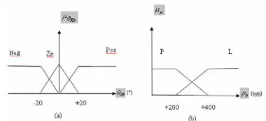
For the «goal seeking» behaviour, we consider three membership functions for the input
Rb
θ (robot-goal angle), and two membership functions for the input ρb (robot-goal distance) (Fig. 3). The knowledge base consists of six fuzzy rules. The FIS controller has two output for the actor, rotation speed Vrot and the translation speed Vit.
Figure 3:membership functions forθRb (a) and ρb (b) From the heuristic nature of FQL algorithm, we carried out several tests to determine the values of the parameters which accelerate the training speed and to obtain good performances for the apprentice. After a series of experiments, we found the following values:
, 9 . 0 , 50 ′=
=
λ
θ
, sp=0.1 and γ =0.9Available actions for all rules, are as follow {-20°/s, -10°/s, -5°/s, 0°/s, +5°/s, +10°/s, +20°/s} for the rotation velocity and {0 mm/s, 150 mm/s, 350mm/s} for translation, which gives 21 possible actions in each fuzzy rule.
The reinforcement function is defined as follows:
- If the robot is far from the goal, the reinforcement is equal to
• 1 if (θRb.
Rb
θ& < 0) & Vit=0
• 1 if (-1°<θRb<+1°) & Vit≠ 0
• 0 if (θRb.
Rb
θ& = 0) & Vit=0
• -1 else
- If the robot is close to the goal, the reinforcement is equal to
• 1 if (θRb.θ&Rb< 0) & Vit=0
• -1 else
Figure (4) shows the trajectory of the robot during the training and validation phase.
Figure 4: Trajectory of the robot during and after training
B. The «obstacle avoidance» behavior
[image:4.595.67.271.320.519.2]For this behaviour, we have determined the translation speed of the robot proportional to the distance from the frontal obstacles, with a maximum value of 350 mm/s “Fig.5”.
[image:4.595.344.523.495.567.2] [image:4.595.337.518.657.716.2]The inputs of the fuzzy controller for this behaviour are the minimal distances provided by the four sets of sonar {min(d90,d50), min(d30,d10), min(g10,g30), min(g90,g50)}, with respectively three membership functions for each one “Fig. 6”.
Figure 6:input membership functions for the fuzzy controller Vrot (a) :{min(d90,d50), min(g90,g50)}
(b) :{min(d10,d30), min(g10,g30)},
The set of the action U common to all rules consists of five actions {-20°/s, -10°/s, 0°/s, +10°/s, +20°/s}.
The reinforcement function is defined as follows:
• +1 if min {min(d90,d50),min(d30,d10)} < min {min(g10,g30),min(g90,g50)} & Vrot > 0
• +1 if min {min(d90,d50),min(d30,d10)}> min {min(g10,g30),min(g90,g50)} & Vrot < 0
•-1 otherwise
[image:5.595.49.276.140.241.2]The figure (7) shows the evolution of the robot during the training phase.
Figure 7:Trajectories of the robot during and after training
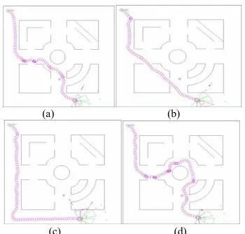
On the following figure, we represent the time evolution of the robot. It shows that the robot is able to be released from the tight corners and deadlock obstacles shape.
(a) (b)
(c) (d)
Figure 8: Time evolution of the robot after training
C. Fusion of the two behaviors
The goal of the two elementary behaviors fusion is to allow the robot navigation in environments composed by fixed obstacles of convex or concave type and to achieve a fixed goal while ensuring its safety, which is a fundamental point in reactive navigation.
The suggested solution consists in considering the whole input variables of the two behaviours « goal seeking » and « obstacle avoidance » associated with distributed reinforcement function by the means of a weighting coefficient between the two behaviours (0.7 for obstacles avoidance and 0.3 for the goal seeking).
The fuzzy controller input are six who are the minimal distances provided by the four sets of sonar {min(d90,d50), min(d30,d10), min(g10,g30), min(g90,g50)}, with respectively three membership functions for the side sets and two membership functions for the frontal sets, to which we add the input
θ
Rb with three membership functions, and ρb with twomembership functions. The rules base thus consists of 216 fuzzy rules; manually it is difficult to ensure conclusion coherence. The translation speed of the robot is proportional to the distance from the frontal obstacles. The FQL algorithm parameters are slightly modified as follows: θ=20 &sp =0.9
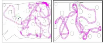
Figure (9) represents the type of trajectory obtained during the training phase. The robot manages to avoid the obstacles and to achieve the goal assigned in environments encumbered by maintaining a reasonable distance between the obstacle and it’s with side dimensions.
Figure (10) illustrates the satisfying behaviour of the robot after training. The various trajectories obtained for the same environment and the same arrival and starting points are due primarily to the problems of the perception of the environment by the robot and are related to the phenomena of sonar readings, these differences confirm at the same time the effectiveness of the training algorithm.
[image:5.595.76.259.471.547.2]
Figure 9: Trajectories of the robot in training phase
400 800 1200 500 900 1400
P M L P M L
[image:5.595.87.252.616.693.2] [image:5.595.335.522.633.707.2](a) (b)
[image:6.595.81.256.81.248.2](c) (d)
Figure 10: Various trajectories of the robot after training
The following figure illustrates the satisfying behaviour of the real robot which evolves/moves in an unknown environment and which manages to achieve the fixed goal.
Figure 11: Trajectory of the real robot after training
V. CONCLUSION
FQL Algorithm makes it possible to introduce generalization into states and actions space, and a conclusions adaptation incrementally of a zero order Sugeno type FIS and this only by the means of the interactions between the apprentice and his environment. The reinforcement function constitutes the measure of the performance of the required behaviour solution. With the FQL algorithm we can solve decision problems in Fuzzy Inference System conclusions. Also, fusion of the behaviours « goal seeking» and « obstacle avoidance » is presented by using a combined reinforcement function. The simulation and experimentation results in various environments are satisfactory.
VI. REFERENCES
[1] S. Babvey, O. Momtahan, M. R. Meybodi, “ Multi Mobile Robot Using Distributed Value function Reinforcement Learning”, IEEE, International Conference on Robotics &Automation, September 2003. [2] H.R. Beom, H. S. Cho, “ A Sensor-Based Navigation for a Mobile Robot
Using Fuzzy Logic and Reinforcement Learning ”, IEEE, Transactions on Systems Man and Cybernetics , vol.25, NO.3 ,pp.464-477, March 1995.
[3] G. Faria, R. A.F Romero “Incorporating Fuzzy Logic to Reinforcement Learning”, IEEE, pp.847-852 ,Brazil,2000.
[4] T. Fujii, Y. Arai , H. Asama, I. Endo, “Multilayered Rienforcement Learning For Complicated collision Avoidance problems”, Proceedings of IEEE, International Conference on Robotics &Automation, pp.2186-2191,May 1998.
[5] T. Fukuda, Y. Hasegawa, K. Shimojima, F. Saito,“Reinforcement Learning Method For Generating Fuzzy Controller”, Department of Micro system Engineering, Nagoya University, pp.273-278, Japan, IEEE, 1995.
[6] P. Y. Glorennec, “Reinforcement Learning: An Overview”, INSA de Rennes ESIT’2000, Aachen, pp.17-35, Germany, September 2000. [7] L. Jouffe, “Apprentissage de Système D’inférence Floue par des
Méthodes de Renforcement”, Thèse de Doctorat, IRISA, Université de Rennes I, Juin 1997.
[8] K. G. KONOLIGE ‘Saphira Référence’, Edition Doxygen, Novembre 2002.
[9] K. G. KONOLIGE ‘Saphira Robot Control Architecture’, Edition SRI International, Avril, 2002
[10] W. D. Smart, L. P. Kaelbling , “ Effective Reinforcement Learning For Mobile Robots”, Proceedings of the IEEE, International Conference on Robotics &Automation, pp.3404-3410, May 2002.
[11] R.S. Sutton, A. Barto, “Reinforcement Learning”, Bradford Book, 1998. [12] C. J. C. H. Watkins, “Learning from delayed rewards”, Ph.D. thesis,
Cambridge University, 1989.
[13] C. Watkins, P. Dayan, “Q-Learning Machine Learning”, pp.279-292, 1992.
[image:6.595.64.271.321.496.2]