Abstract—In this paper, we propose a novel recurrent interval type-2 fuzzy neural network with asymmetric membership functions (RT2FNN-A). The RT2FNN-A uses the interval asymmetric type-2 fuzzy sets and it implements the fuzzy logic system (FLS) in a five-layer neural network structure. The RT2FNN-A is modified from the type-2 fuzzy neural network to provide memory elements for capturing the system’s dynamic information and has the properties of high approximation accuracy and small network structure. Based on the Lyapunov theorem and gradient descent method, the convergence of RT2FNN-A is guaranteed and the corresponding learning algorithm is derived. In addition, the RT2FNN-A is applied in the nonlinear channel equalization to show the performance and effectiveness of RT2FNN-A system.
Index Terms—type-2 fuzzy logic system, recurrent neural network, asymmetric membership functions, channel equalization
I. INTRODUCTION
In recent years, the fuzzy systems and control are regarded as the most widely used application of fuzzy logic system [5-9, 22]. Mendel and Karnik developed a complete theory of type-2 fuzzy logic systems (T2FLSs) [8, 16, 21-22]. Recently, T2FLSs have attracted more attention in many literatures and special issues [1, 6, 10-11, 16, 21-22, 24].
The major difference being the present of type-2 is their antecedent and consequent sets. T2FLSs result in better performance than type-1 fuzzy logic systems on the applications of function approximation, modeling, and control. Besides, neural networks have found numerous practical applications, especially in the areas of prediction, classification, and control [15]. Based on the advantages of T2FLSs and neural networks, the type-2 fuzzy neural network (T2FNN) systems are presented to handle the system uncertainty and reduce the rule number and computation [1, 10-11, 22, 24]. Using the asymmetric Gaussian function which is a new type of membership function due to excellent approximation results it provides. It also provides a fuzzy-neural network with higher flexibility to easily approach the optimum result more accurately. In the literature [9-10, 23], a T2FNN with asymmetric membership functions (T2FNN-A) was proposed to improve the system performance and obtain better approach ability.
In recent years, the nonlinear channel equalization using intelligent system was discussed [1-2, 17, 19-20]. Literature [4] introduced the ionospheric scintillation phenomenon
This work was supported in part by the National Science Council,
Taiwan, R.O.C., under contracts NSC-95-2221-E-155-068-MY2.
Ching-Hung Lee is with Department of Electrical Engineering, Yuan-Ze University, Chung-li, Taoyuan 320, Taiwan. (phone: +886-3-4638800, ext: 7119; fax: +886-3-4639355, e-mail: [email protected]).
which may cause multi-path problem when signal was transmitted. The multi-path problem is similar to nonlinear time-varying channel. In [19], there were successful application cases in complex channel equalization by using self-constructing fuzzy neural network, but a larger fuzzy rule number should be used when signal to noise ratio is low.
In this paper, we proposed a combining interval type-2 fuzzy asymmetric membership functions with recurrent neural network system, called RT2FNN-A. The proposed RT2FNN-A is a modified version of the T2FNN [11-14, 20, 24] which provides memoried elements to capture system dynamic response [15]. The RT2FNN-A system capability for temporarily storing information allowed us to extend the application domain to include temporal problem. Simulations are shown to illustrate the effectiveness of the RT2FNN-A system.
II. INTERVAL TYPE-2 FUZZY NEURAL NETWORK SYSTEMS
We first introduce the recurrent type-2 neural fuzzy inference system with asymmetric fuzzy MFs (RT2FNN-A) that was modified and extended from previous results [4, 5, 8, 12]. The RT2FNN-A uses the interval asymmetric type-2 fuzzy sets and it implements the FLS in a five-layer neural network structure which contains four-layer forward network and a feedback layer.
-3 -2 -1 0 1 2 3
0 0.2 0.4 0.6 0.8 1
Lower MFs
-3 -2 -1 0 1 2 3
0 0.2 0.4 0.6 0.8 1
Upper MFs
) (l σ σ(r)
) (l σ
) (r σ
) (l
m (r)
m (l)
m (r)
m
) (x
μ μ(x)
[image:1.595.318.534.455.662.2](c)
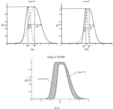
Figure 1: Construction of a type-2 AFMF: (a) upper MF (solid line), (b) lower MF (solid line), and (c) constructed type-2 AFMF.
A. Construction of Type-2 Asymmetric Fuzzy Membership Functions
In general, given an system input data set xi, i=1, 2, …, n,
and the desired output yp, p=1, 2, …, m, the jth type-2 fuzzy
rule has the form
Ching-Hung Lee, Member, IAENG, Hao-Han Chang, Che-Ting Kuo, Jen-Chieh Chien, and Tzu-Wei Hu
A Novel Recurrent Interval Type-2 Fuzzy Neural
Rule j: IF x1 is F1j
~
and … xn is Fnj ~
THEN y1 is
j
w~ and …1 ym is j m
w~
where j is the number of rules, j i
F~ represents the linguistic term of the antecedent part, j
p
w~ represents the real number of
the consequent part; n and m are the numbers of the input and output dimensions, respectively. Besides, the representation of jth rule for RT2FNN-A is
Rule j: IF x1 is G1j
~
and … xn is Gnj
~
and gj is GFj
~
THEN y1 is
j
w~ and … 1 ym is j m
w~ , g1 is
j
a~1, g2 is
j
a2
~ , …, and g
M is
j M
a
~ . where Gij
~
represents the linguistic term of the antecedent part,
j p
w~ and j p
a
~ represents the interval real number of the consequent part; and M is the rule number. Here the fuzzy MFs of the antecedent part Gij
~
are asymmetric interval type-2 fuzzy sets, which represent the different from typical Gaussian MFs.
Here we use the superscripts (l) and (r) to denote the left and right curves of a Gaussian MF. The parameters of lower and upper MFs are denoted by an underline (_) and bar ( ), respectively. Thus, the upper MF is constructed as
⎪ ⎪ ⎪ ⎪ ⎩ ⎪⎪ ⎪ ⎪ ⎨ ⎧ ≤ ⎥ ⎥ ⎦ ⎤ ⎢ ⎢ ⎣ ⎡ ⎟⎟ ⎠ ⎞ ⎜⎜ ⎝ ⎛ − − ≤ ≤ ≤ ⎥ ⎥ ⎦ ⎤ ⎢ ⎢ ⎣ ⎡ ⎟⎟ ⎠ ⎞ ⎜⎜ ⎝ ⎛ − − = x m m x m x m m x m x x r r r r l l l l F ) ( 2 ) ( ) ( ) ( ) ( ) ( 2 ) ( ) ( ~ for , 2 1 exp for , 1 for , 2 1 exp ) ( σ σ
μ (1)
where (l)
m and (r)
m denote the means of two Gaussian MFs satisfying (l) (r)
m
m ≤ , and σ(l)
and σ(r)
denotes the deviation (i.e., width) of two Gaussian MFs. Figure 1(a) shows the upper type-2 AFMF constructed using (l)
m , (r)
m ,
) (l
σ , and σ(r)
. Similarly, the lower asymmetric MF is defined as ⎪ ⎪ ⎪ ⎪ ⎩ ⎪⎪ ⎪ ⎪ ⎨ ⎧ ≤ ⎥ ⎥ ⎦ ⎤ ⎢ ⎢ ⎣ ⎡ ⎟⎟ ⎠ ⎞ ⎜⎜ ⎝ ⎛ − − ⋅ ≤ ≤ ≤ ⎥ ⎥ ⎦ ⎤ ⎢ ⎢ ⎣ ⎡ ⎟⎟ ⎠ ⎞ ⎜⎜ ⎝ ⎛ − − ⋅ = x m m x r m x m r m x m x r x r r r r l l l l F ) ( 2 ) ( ) ( ) ( ) ( ) ( 2 ) ( ) ( ~ for , 2 1 exp for , for , 2 1 exp ) ( σ σ
μ (2)
where m(l)≤m(r) and 0.5≤r≤1 . The corresponding widths of the MFs are σ(l) and σ(r). To avoid unreasonable MFs, the following constrains are added:
. 1 5 . 0 , () () ) ( ) ( ) ( ) ( ) ( ) ( ⎪ ⎪ ⎩ ⎪⎪ ⎨ ⎧ ≤ ≤ ≤ ≤ ≤ ≤ ≤ r m m m m r r l l r r l l σ σ σ
σ (3)
Figure 1(b) sketches the lower type-2 AFMF. The corresponding constructed type-2 AFMF is shown in Fig. 1(c). This introduces the properties of uncertain mean and variance [14]. Additionally, we can construct other type-2 asymmetric MFs by tuning the parameters. The corresponding tuning algorithm is derived to improve system
Layer 1: Input layer Layer 2: Membership layer Layer 3: Rule layer
Layer 4: Output layer
∑ n x 1 x ∏ y ∑ ∑ ∏ 11 ~ G G1M
~
1
~
n G GnM
~ F M G~ F G1 ~ 1 − Z 1 − Z
L L L
L L L
L
] [f1 f1
] [fM fM
] [w1 w1
] [wM wM
] [a11 a11
] [a1M a1M
] [aMM aMM
] [aM1 aM1
Layer 5: Feedback layer
Layer 1: Input layer Layer 2: Membership layer Layer 3: Rule layer
Layer 4: Output layer
Layer 1: Input layer Layer 2: Membership layer Layer 3: Rule layer
Layer 4: Output layer
∑ n x 1 x ∏ y ∑ ∑ ∏ 11 ~ G G1M
~
1
~
n G GnM
~ F M G~ F G1 ~ 1 − Z 1 − Z
L L L
L L L
L
] [f1 f1
] [fM fM
] [w1 w1
] [wM wM
] [a11 a11
] [a1M a1M
] [aMM aMM
] [aM1 aM1
Layer 5: Feedback layer
∑ n x 1 x ∏ y ∑ ∑ ∑∑ ∏ ∏ 11 ~ G G1M
~
1
~
n G GnM
~ F M G~ F G1 ~ 1 − Z 1 − Z
L L L
L L L
L
] [f1 f1
] [fM fM
] [w1 w1
] [wM wM
] [a11 a11
] [a1M a1M
] [aMM aMM
] [aM1 aM1
[image:2.595.305.550.51.215.2]Layer 5: Feedback layer
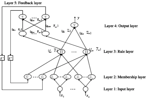
Figure 2: Diagram of MISO recurrent type-2 fuzzy neural network with AFMFs (RT2FNN-A).
III. STRUCTURE OF RECURRENT TYPE-2FUZZY NEURAL
NETWORK WITH ASYMMETRIC MFS (RT2FNN-A)SYSTEM
The RT2FNN-A is shown in Fig. 2. In the following, we use (l)
i
O to denote the ith output of a node in the lth layer. Layer 1: Input Layer
For the ith node of layer 1, the net input and output are represented as
(1) (1) i
i x
O = (4) where (1)
i
x represents the ith input to the jth node. Layer 2: Membership Layer
In layer 2, it is clear that there are two parts in this layer, regular nodes and feedback nodes. Their input are (1)
j
O and )
(k
gj . Therefore, for network input xi, the output is
[
]
[
( ) ( (1))]
.~ ) 1 ( ~ ) 2 ( ) 2 ( ) 2 ( T i G i G T ij ij
ij O O O O
O ij ij μ μ =
= (5)
For internal or feedback variable gj,
[
]
[
G j G j]
TT F j F j F
j O O g k g k
O F j F j )) ( ( )) ( ( ~ ~ ) 2 ( ) 2 ( ) 2
( = = μ μ
(6) where the subscript ij indicates the jth term of the ith input
) 1 ( i
O , where j=1,…, M. The superscript F indicates the feedback layer.
Layer 3: Rule Layer
Using the product t-norm, the firing strength associated with the jth rule is
~ ( 1) ~ ( ) ~ ()
1 ⋅ ∗ ∗ ∗ = jF j j n
j F n G
F j
x x
f μ L μ μ (7) ~ ( 1) ~ ( ) ~ ()
1 ⋅ ∗ ∗ ∗ = jF j j n
j F n G
F j
x x
f μ L μ μ (8) where ~ (⋅)
j
G
μ and ~ (⋅)
j
G
μ are the lower and upper membership grades of ~(⋅)
G
[image:2.595.55.291.330.415.2]Layer 4: Output Layer
Without loss of generality, the consequent part of interval T2FLS is w~j =
[
wj wj]
T, wj ≤wj . The vector notationsT M
w w
w=[ 1 L ] and
T M
w w
w=[ 1 L ] are used for clarity. According to the literature [23], we denote the maximum and minimum of
∑
iM=1fiwi as) 4 (
O and O(4).
(
)
(
)
, 1 ) 3 ( 1 ) 3 ( ) 4 (∑
∑
= + = + = = M L j j j L j j j L T w O w O f wO (10)
∑
(
)
∑
(
)
+ = = + = = M R j j j R j j j R T w O w O f w O 1 ) 3 ( 1 ) 3 ( ) 4 ( (11) where[
]
[
]
TM L L T M L L
L f f f f O O O O
f (3) (3) (3)1 (3)
1 1
1,L, , +,L, = ,L, , +,L,
=
(12)
[
, , , , ,]
[
, , , (3), , (3)]
1 ) 3 ( ) 3 ( 1 1 1 T M R R T M R R
R f f f f O O O O
f = L + L = L + L .
(13) It is obvious that R and L should be calculated first. The weights are arranged in order as w1≤w2≤LwM and
M
w w
w1≤ 2 ≤L . According to the Karnik-Mendel procedure [8, 16, 22], L and R are
( )
, minarg (4)
] 1 , . 1 [ O L M
j∈ −
= L
arg max
( )
(4) .] 1 , . 1 [ O R M
j∈ −
= L
(14) Finally, the crisp output is
. 2 ) 4 ( ) 4 ( ) 4
( O O
O = + (15)
Layer 5: Feedback Layer
This layer contains the context nodes which is used to produce the internal or feedback variable gj. Each rule is
associated with a particular internal variable. Hence, the number of the context nodes is equal to the number of rules. The same operations (type-reduction and defuzzification) as layer 4 are performed here.
(
)
∑
(
)
∑
+ = = + = = + M L h jh h L h jh h L T j j F j F j a O a O f a k O 1 ) 3 ( 1 ) 3 ( ) 5 ( ) 1( (16)
(
)
∑
(
)
∑
+ = = + = = + M R h jh h R h jh h R T j j F j F j a O a O f a k O 1 ) 3 ( 1 ) 3 ( ) 5 ( ) 1( (17)
and
(
( 1))
, minarg (5)
] 1 , . 1 [ + = −
∈ O k
L j M h F j L (18)
(
( 1))
.max
arg (5)
] 1 , . 1 [ + = − ∈ k O R j M h F j L (19) Finally, the crisp output of this layer is
[
( 1) ( 1)]
.2 1 ) 1 ( ) 1
(k+ =O(5) k+ = O(5) k+ +O(5) k+
gj j j j (20)
Note that the delayed value of gj is fed into layer 2, and it
acts as an input variable to the precondition part of a rule. Each fuzzy rule has the corresponding internal variable gj
which is used to decide the influence degree of temporal history to the current rule.
A. Learning Algorithm for RT2FNN-A System
The gradient descent method is adopted to derive learning algorithm of the RT2FNN-A system. For clarification, we consider the single-output system and define the error cost function as
2 )] ( ˆ ) ( [ 2 1 )
(k y k yk
E = d − (21)
where yd is the desired output and yˆ is the RT2FNN-A’s
output. Using the gradient descent algorithm, the parameters updated law is
⎟⎟ ⎠ ⎞ ⎜⎜ ⎝ ⎛ ∂ ∂ − + = Δ + = + ) ( ) ( ) ( ) ( ) ( ) 1 ( k k E k k k k W W W W
W η (22)
in which η is the learning rate ( 0<η≤1 ).
]
[ F F a F
w W W W W W r r
W
W= are the
adjustable parameters, where Ww is consequent weights, W
and WF are parameters of lower MFs, W and WF
are upper MFs parameters, Wa is parameter in feedback layer,
and r and rF are the column vectors, i.e.,
[
]
Tw = w w
W
(23)
[
]
Ta = a a
W (24)
[
l r l r]
Tm
m() () σ() σ( )
=
W (25)
[
l r l r]
Tm
m() ( ) σ() σ()
=
W (26)
[
Fl Fr Fl Fr]
TF
m
m () () σ () σ ( )
=
W (27)
[
Fl Fr Fl Fr]
TF
m
m () () σ () σ ()
=
W . (28)
Considering ∂E(k) ∂W(k), we have
[
]
. ) ( ) ( ˆ ) ( ˆ ) ( ) ( ) ( ˆ ) ( ˆ ) ( ) ( ) ( k k y k y k y k k y k y k E k k E d W W W ∂ ∂ − − = ∂ ∂ ∂ ∂ = ∂ ∂(29) Thus, (21) can be rewritten as
) ( ) ( ˆ ) ( ) ( ) 1 ( k k y k e k k W W W ∂ ∂ + =
+ η
(30)
where e(k)= yd(k)−yˆ(k). The remaining work involves finding the corresponding partial derivative with respect to each parameter.
Observing equation (16) and if j≤L, only the term of
(
)
∑
=L
j1Oj wj ) 3 (
should be considered, and only consider
(
)
∑
= +M
L
j 1Oj wj
) 3 (
if j>L . Moreover, we consider
(
)
∑
=R
j1Oj wj ) 3 (
if j≤R in (17), as well as
∑
Mj=R+1(
Oj wj)
) 3 (where j>R. Thus, we should notice the values of j, R, and L
in deriving the update laws.
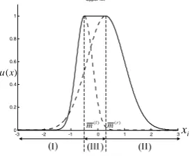
In order to avoid unnecessary tuning, we must also consider the firing regions of MFs for input variable xi. For
example, considering an upper MF as shown in Fig. 3, region (I)- (l)
ij
i m
x ≤ , only (l) ij
m and (l) ij
σ are updated; region (II)-
i r
ij x
m( )≤
, only (r) ij
m and (r) ij
σ must be updated as well. Finally, region (III)- () (r)
ij i l
ij x m
Besides, parameter
r
must be updated for all three regions. Owing the recurrent property, the real time recurrent learning algorithm (RTRL) is used [26]. The update rules of RT2FNN-A can be derived. Herein, we omit them due to the limitation of writing space.-3 -2 -1 0 1 2 3
0 0.2 0.4 0.6 0.8 1
Upper MFs
) (l
m (r)
m
i
x )
(x
[image:4.595.111.248.120.233.2]μ
Figure 3: Firing regions definition of input variable xi (upper MF).
B. Stability Analysis of RT2FNN-A System
By [3, 15, 23], using the Lyapunov stability approach, we have the following convergence theorem.
Theorem 1: Let [ηw ηa η η ηr] be the learning rates of the tuning parameters for RT2FNN-A. The asymptotic convergence of RT2FNN-A is guaranteed if proper learning rates [ηw ηa η η ηr] are chosen
satisfying the following condition.
(
+ + + + + + + + rF)
<2F F a a r
w λ λ λ λ λ λ λ λ
λ (31)
Proof: The proof is omitted due to the limitation of writing space.
IV. NONLINEAR CHANNEL EQUALIZATION USING
RT2FNN-ASYSTEM
To demonstrate the performance of RT2FNN-A system, several simulations regarding signal processing are constructed. The RT2FNN-A system is applied to nonlinear time-varying channel equalization to overcome the multi-path problem when signal is transmitted.
A. Nonlinear Channel Equalization
The channel characteristic represents random temporal fluctuations by the time-varying amplitude factor. The received signal can be described as follows
) ( ) 1 (
... ) 1 ( ) ( ) (
ˆ t c1st c2st c s k p nk
x = + − + + p − + + (32)
where s(t) is transmitted signal, and xˆ(t) denotes the channel state; cl, l=1,2,...,p, are time-varying amplitude factor, and
p is the channel order. The channel characteristic is similar to nonlinear time-varying channel. In order to reduce multi-path channel interference, we firstly introduce nonlinear time-varying channel equalization in next section.
The nonlinear channel equalization is a technique used to combat some imperfect phenomenon in high-speed data transmission over channels [25]. Figure 4 shows the block diagram of a communication system that is subject to inter-symbol interference (ISI) and additive white Gaussian noise (AWGN). The transmitted input symbols s(k) is independent and identically distributed discrete-time random processes taking its value {-1, +1}. The signal is sent through
In real communications, the channel is too dispersive to cause interference between successive signal samples (inter-symbol interference). It will complicate reliable transmission and reception. xˆ(k) denotes the output of the channel. The channel function can be described as [20]
(
( ), ( 1), , ( 1))
) (
ˆ k = f sk s k− sk−p+
x L (33)
where p means the channel order. Generally, f is a nonlinear function of past transmitted signals, and the channel changes slowly but significantly over time; therefore, a nonlinear channel equalizer with adaptation ability is
needed. Let T
n k x k x
(k) [ˆ( ), ,ˆ( 1)]
ˆ ≡ ⋅ ⋅⋅ − +
x , where xˆ(k) is
called channel state.
At receiving terminal, the inter-symbol interference and nonlinear distortion are introduced by the channel; received signals x(k) are also assumed to be corrupted by a additive noise n(k), that is
) ( ) ( ˆ )
(k x k n k
x = + (34) where n(k) is an additive white Gaussian noise (AWGN), and is assumed to be zero mean white Gaussian.
D
Equalizer + x(k)
Channel D
x(k-1)
z-1
Equalizer +
n(k)
s(k)
Channel z-1
-x(k-p+1)
) ( ˆk d
s −
z-d
+
-) ( ˆk x
e(k)
D
Equalizer + x(k)
Channel D
x(k-1)
z-1
Equalizer +
n(k)
s(k)
Channel z-1
-x(k--p+1)
x(k-p+1)
) ( ˆk d
s −
z-d
+
-) ( ˆk x
e(k)
Figure 4: Block diagram of adaptive equalizer.
The function of the equalizer is to re-construct the transmitted signal, s(k−d) (d denotes the decision delay), from the observed information sequence,
) 1 (
, ),
(k xk−p+
x L from which greater speed and reality can be achieved. Thus, the mathematical representation of equalizer is
)) 1 (
, ), 1 ( ), ( ( ) (
ˆ k−d = xk x k− ⋅⋅⋅ x k−p+
s ψ (35)
where ψ :ℜp→{1,−1}
. We can say that a correct decision by the equalizer if
) ( ) (
ˆk d sk d
s − = − . (36) Based on the category of s(k−d) (i.e., 1± ), the channel states xˆ(k) can be partitioned into two classes [2]
{
ˆ( )| ( − )=1}
,=
+
d k s k x
X (37) X− =
{
xˆ(k)|s(k−d)=−1}
. (38) The numbers of elements in X+ and X− are denoted as ns+and ns−, respectively [2]. The probabilities for s(k−d)=1
and s(k−d)=−1 are the same, which means,
2 / s s
s n n
n+ = − = , where ns is the total number of channel
state. Besides, the channel states in X+ and X− are denoted )
, , 1 (
ˆi+ i= ns+
[image:4.595.320.542.312.456.2]Suppose channel order is p=2 in the nonlinear channel function. For a time-varying channel, the coefficients of the channel, ci, i=0, 1,K,n, are unknown. The nonlinear time-varying channel model is described as [18, 20]
) ( ) ( ) 1 ( ) ( )
(k c1s k c2s k H k n k
x = + − − + (39)
where c1 and c2 are time-varying coefficients, and H(k) is
Co-Channel Interference, (CCI) is described as ) ) ( ) ( ( )
( 1
12 11
−
+
= c k c k z
z
H λ (40) where c11(k) and c12(k) are co-channel time-varying
coefficients.
The time-varying coefficients, c1 and c2, are simulated by
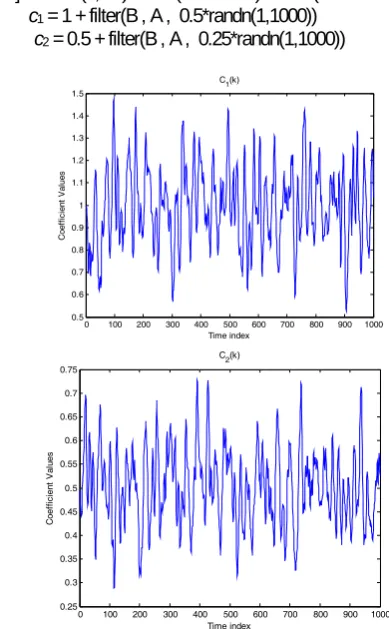
using a second-order Markov model. It is also called second-order Butterworth low-pass filter (LPF) which is derived by white Gaussian noise source [18]. In our simulations below, we use the function butter, provided by the Matlab- Signal Processing Toolbox, to generate a second-order low-pass digital Butterworth filter with cutoff frequency 0.1. Then the function filter is used to generate a colored Gaussian sequence, which is then used as time-varying channel coefficients. Note that we center c1(k) around 1 and c2(k) around 0.5 as shown in Fig. 5. The input to Butterworth filter is a white Gaussian sequence code for time-varying coefficients with length of 1000. The Matlab codes are [18]
[B, A] = butter(2,0.1) % B (numerator) and A (denominator) of LPF c1 = 1 + filter(B , A , 0.5*randn(1,1000))
c2 = 0.5 + filter(B , A , 0.25*randn(1,1000))
0 100 200 300 400 500 600 700 800 900 1000 0.5
0.6 0.7 0.8 0.9 1 1.1 1.2 1.3 1.4 1.5
Time index
Coef
fic
ient
V
al
ues
C1(k)
0 100 200 300 400 500 600 700 800 900 1000 0.25
0.3 0.35 0.4 0.45 0.5 0.55 0.6 0.65 0.7 0.75
Time index
C
oef
fic
ien
t V
al
ues
[image:5.595.305.550.50.167.2]C2(k)
Figure 5: Time-varying channel coefficients.
Time-varying channel )
(k s
+ ) (k n
Type-2 FNN )
(k x
Learning Algorithm
d
Z−
+ −
) ( ˆk d s −
) (k d s −
Error
Time-varying channel )
(k s
+ ) ( ˆk
x x(k)
Learning Algorithm
d
z−
+ −
) ( ˆk d s −
) (k d s −
Error
RT2FNN-A Time-varying
channel )
(k s(k)
s
+ ) (k n
Type-2 FNN )
(k x(k)
x
Learning Algorithm
d
Z−d Z−
+ −
) ( ˆk d sˆ(k−d)
s −
) (k d s(k−d)
s −
Error
Time-varying channel )
(k s(k)
s
+ ) ( ˆk xˆ(k)
x xx((kk))
Learning Algorithm
d
z−d z−
+ −
) ( ˆk d sˆ(k−d)
s −
) (k d s(k−d)
s −
Error
[image:5.595.57.252.383.698.2]RT2FNN-A
Figure 6: Block diagram of adaptive equalizer using RT2FNN-A system.
Herein, we use the RT2FNN-A system to be an adaptive equalizer for time-varying channel equalization. As Fig. 6 shows, we use the RT2FNN-A filter to construct the equalizer and take the error to update the parameters of RT2FNN-A filter which can achieve the adaptive equalizer. In our simulations, we choose the independent input sequence s(k) which consists of 2000 symbols. The first 1000 symbols are used for training, and the remaining 1000 are used for testing. After training, the parameters of the T2FNN, T2FNN-A and RT2FNN-A filters are fixed, and then the testing is performed. Then, we compare two examples among these three types of filters.
Firstly, we do not consider the CCI, i.e., H(k)=0. We assume that the time-varying channel is the form of (39) and we choose 4 rules to construct the RT2FNN-A filter. The learning rate is chosen to be 0.1, whereas the training epoch is 50. Figure 7 shows the simulation results (solid-line: RT2FNN-A, dashed-line: T2FNN-A, and dotted-line: T2FNN). The comparisons of network structure and bit error rate (BER) are shown in Table 1. Obviously, the performance using our approach is also better than T2FNN-A and T2FNN (smaller BER value).
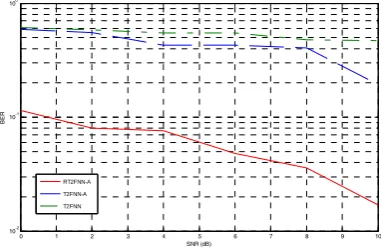
Next, we consider the time-varying channel with the co-channel for CCI [20]
3 1 12
11( ) ( ) )
( 9 . 0 )
(z = ⋅ c k +c k z−
H (41) where the nominal values are c11(k)=1 and c12(k)=0.5.
The learning rate is set as 0.1, whereas the training epoch is 50. Figure 8 shows the simulation results (solid-line: RT2FNN-A, dashed-line: T2FNN-A, and dotted-line: T2FNN). We found that the performance is better than T2FNN-A and T2FNN (smaller BER value). We can see that our approach results better performance and has advantages of fewer adjustable parameters and smaller BER value.
0 1 2 3 4 5 6 7 8 9 10
10-3 10-2 10-1 100
SNR (dB)
BE
R
RT2FNN-A T2FNN-A T2FNN
Figure 7: Performance comparisons of nonlinear time-varying channel without CCI (solid-line: RT2FNN-A, dashed-line: T2FNN-A, and
[image:5.595.333.521.597.722.2]0 1 2 3 4 5 6 7 8 9 10 10-2
10-1 100
SNR (dB)
BER
RT2FNN-A T2FNN-A T2FNN
Figure 8: Performance comparisons of nonlinear time-varying channel with CCI (solid-line: RT2FNN-A, dashed-line: T2FNN-A, and dotted-line:
[image:6.595.73.264.59.183.2]T2FNN).
Table 1: Comparison results of network structure, rule number, parameter number, and BER for Example 1 (SNR=10 dB).
BER Network
structure
Rule No.
(M) Parameter No Without
CCI
With CCI
2-30-15-1 15 120 0.1897 0.4704
T2FNN[29]
2-8-4-1 4 32 0.597 0.798
2-18-9-1 9 108 0.0825 0.1932
T2FNN-A[37]
2-8-4-1 4 48 0.434 0.601
RT2FNN-A 2-8-4-1 4 100 0.0063 0.017
V. CONCLUSION
In this paper, we propose a recurrent interval type-2 fuzzy neural network with asymmetric membership functions (RT2FNN-A). The novel RT2FNN-A uses the interval asymmetric type-2 fuzzy sets implements the FLS in a five-layer neural network structure which contains four-layer forward network and a feedback layer. According to the Lyapunov theorem and gradient descent method, the convergence of RT2FNN-A is guaranteed and the corresponding learning algorithm is derived. The effect of RT2FNN-A has been introduced by several illustration examples.
From the simulation results, a RT2FNN-A equalizer over various channel models are presented in this paper. Simulation results have been carried out in both real-valued and complex-valued nonlinear channels to ensure the flexibility of the proposed equalizer. The feedback layer of proposed RT2FNN-A makes it have advantages of storing past information. Moreover, the RT2FNN-A can use a small number of tuning parameters than the feed-forward fuzzy neural networks to obtain better performances (smaller BER). To reduce the computation complexity, RT2FNN-A is a good choice.
REFERENCES
[1] O. Castillo and P. Melin, “Adaptive Noise Cancellation Using Type-2
Fuzzy Logic and Neural Networks,” IEEE International Conf. on Fuzzy
Systems, Vol. 2, pp. 1093-1098, 2004.
[2] S. Chen, B. Mulgrew, and S. McLaughlin, “A Clustering Technique for
Digital Communication Channel Equalization Using Radial Basis
Function Network,” IEEE Trans. on Neural Networks, Vol. 4, No. 2, pp.
570-579, 1993.
[3] Y. C. Chen and C. C. Teng, “A Model Reference Control Structure
Using A Fuzzy Neural Network,” Fuzzy Sets and Systems, Vol. 73, pp.
291-312, 1995.
[4] R. K. Crane, “Ionospheric Scintillation,” Proc. of IEEE, Vol. 65, No. 2,
pp. 180-199, 1977.
[5] J. S. Jang, “ANFIS: Adaptive-network-based Fuzzy Inference System,”
IEEE Trans. on Systems, Man, and Cybernetics, Vol. 23, No. 3, pp.
665-685, 1993.
[6] R. John and S. Coupland, “Geometric Type-1 and Type-2 Fuzzy Logic
Systems,” IEEE Trans. on Fuzzy Systems, Special Issue on Type-2 Fuzzy
Systems, Vol. 15, No. 1, pp. 3-15, 2007.
[7] C. F. Juang, ”A TSK-Type Recurrent Fuzzy Network for Dynamic
Systems Processing by Neural Network and Genetic Algorithms,” IEEE
Trans. on Fuzzy Systems, Vol. 10, No. 2. pp. 155-170, 2002.
[8] N. N. Kamik, J. Mendel, and Q. Liang, “Type-2 Fuzzy Logic Systems,”
IEEE Trans. on Fuzzy Systems, Vol. 7, No. 6, pp. 643-658, 1999.
[9] C. H. Lee and H. Y. Pan, “Enhancing the Performance of Neural Fuzzy
Systems Using Asymmetric Membership Functions,” Revised in Fuzzy
Sets and Systems, 2007.
[10] C. H. Lee and H. Y. Pan, “Construction of Asymmetric Type-2 Fuzzy
Membership Functions and Application in Time Series Prediction,”
International Conf. on Machine Learning and Cybernetics, Vol. 4, pp.
2024-2030, 2007.
[11] C. H. Lee and Y. C. Lin, “An Adaptive Type-2 Fuzzy Neural Controller
for Nonlinear Uncertain Systems,” International Journal of Control and
Intelligent, Vol. 12, No. 1, pp. 41-50, 2005.
[12] C. H. Lee and Y. C. Lin, “Control of Nonlinear Uncertain Systems
Using Type-2 Fuzzy Neural Network and Adaptive Filter,” IEEE
International Conf. on Networking, Sensing, and Control, Vol. 2, pp.
1177-1182, 2004.
[13] C. H. Lee, Y. C. Lin, and W. Y. Lai, “Systems Identification Using
Type-2 Fuzzy Neural Network (Type-2 FNN) Systems,” IEEE
International Sym. on Computational Intelligence in Robotics and
Automation, Vol. 3, pp. 1264-1269, 2003.
[14] C. H. Lee, J. L. Hong, Y. C. Lin, and W. Y. Lai, “Type-2 Fuzzy Neural
Network Systems and Learning,” International Journal of
Computational Cognition, Vol. 1, No. 4, pp. 79-90, 2003.
[15]C. H. Lee and C. C. Teng, “Identification and Control of Dynamic
Systems Using Recurrent Fuzzy Neural Networks,” IEEE Trans. on
Fuzzy Systems, Vol. 8, No. 4, pp. 349-366, 2000.
[16]A. Q. Liang and J. M. Mendel, “Interval Type-2 Fuzzy Logic Systems:
Theory and Design,” IEEE Trans. on Fuzzy Systems, Vol. 8, No. 5, pp.
535-550, 2000.
[17] A. Q. Liang and J. M. Mendel, “Overcoming Time-varying Co-channel
Interference Using Type-2 Fuzzy Adaptive Filters,” IEEE Trans. on
Circuits and Systems, Vol. 47, No. 12, pp. 1419-1428, 2000.
[18] A. Q. Liang and J. M. Mendel, “Equalization of Nonlinear
Time-varying Channels Using Type-2 Fuzzy Adaptive Filters,” IEEE
Trans. on Fuzzy Systems, Vol. 8, No. 5, pp. 551-563, 2000.
[19]R. C. Lin, W. D. Weng and C. T. Hsueh, “Design of An SCRFNN-based
Nonlinear Channel Equaliser,” IEE Proc. Communications, Vol. 152, No.
6, pp. 771-779, 2005.
[20] Y. C. Lin, Type-2 Fuzzy Neural Network System and Its Applications in
Signal Processing, Nonlinear System Identification, and Control, Master
Paper of Yuan-Ze University, Taiwan, 2004.
[21] J. M. Mendel and R. I. John, “Type-2 Fuzzy Sets Made Simple,” IEEE
Trans. on Fuzzy Systems, Vol. 10, No. 2, pp. 117-127, 2002.
[22]J. M. Mendel, Uncertain Rule-Based Fuzzy Logic Systems: Introduction
and New Directions, Upper Saddle River, Prentice-Hall, NJ, 2001.
[23] H. Y. Pan, Type-2 Fuzzy Neural Network With Asymmetric
Membership Functions Analysis and Its Applications, Master Paper of
Yuan-Ze University, Taiwan, 2006.
[24]C. H. Wang, C. S. Cheng, and T. T. Lee, “Dynamical Optimal Training
for Interval Type-2 Fuzzy Neural Network (T2FNN),” IEEE Trans. on
Systems, Man, Cybernetics Part-B, Vol. 34, No. 3, pp. 1462-1477, 2004.
[25] R. J. Williams and D. Zipser, “A Learning Algorithm for Continually
Running Recurrent Neural Networks,” Neural Computation, Vol. 1, No.
2, pp. 270-280, 1989.
[26]L. A. Zadeh, “The Concept of A Linguistic Variable and Its Application
to Approximate Reasoning,” Information Sciences, Vol. 8, No.3, pp.