Double Barrier Hitting Time Distribution of a Mean-reverting
Lognormal Process and Its Application to Pricing Exotic Options
∗
C.F. Lo
†‡, T.K. Chung
§and C.H. Hui
¶Abstract
In this paper we propose a simple and easy-to-use method for computing accurate estimate (in closed form) of the double barrier hitting time distribution of a mean-reverting lognormal process, and discuss its application to pricing exotic options whose payoffs are contingent upon barrier hitting times. This new ap-proach is also able to provide tight upper and lower bounds (in closed form) of the exact result. Within the multi-stage approximation scheme, the estimate and bounds can be easily improved in a systematic manner. Furthermore, this approach can be straight-forwardly extended to those cases with specified mov-ing boundaries as well.
Keywords: First hitting time; mean-reverting lognor-mal process; barrier options; method of images.
1. Introduction
In the past decade barrier options have become very popular instruments for a wide variety of hedging and investment in foreign exchange, equity and com-modity markets, largely in the over-the-counter mar-kets. An advantage of trading barrier options is that they provide moreflexibility in tailoring the portfolio
∗The conclusions herein do not represent the views of the Hong Kong Monetary Authority.
†Author for correspondence. Institute of Theoretical
Physics and Department of Physics, The Chinese University of Hong Kong, Shatin, New Territories, Hong Kong, China (Email: [email protected])
‡Hong Kong Institute for Monetary Research, Hong Kong
Monetary Authority, 55th Floor, Two International Finance Centre, 8 Finance Street, Hong Kong, China
§Department of Physics, The Chinese University of Hong
Kong, Shatin, New Territories, Hong Kong, China (Email: [email protected])
¶Research Department, Hong Kong Monetary Authority,
55th Floor, Two International Finance Centre, 8 Finance Street, Hong Kong, China (Email: [email protected])
returns while lowering the cost of option premiums. In the commodity and foreign exchange markets em-pirical studies show that the mean-reverting lognor-mal process (MRL-process) provides a more accurate description of the commodity prices and exchange rates than the lognormal process. However, unlike the standard barrier options for a lognormal process, the valuation of barrier options for a MRL-process poses a real challenge for there is no exact analytical solution available (Lo and Hui 2006).
Recently, based upon the method of images, Hui and Lo (2006) were able to develop an efficient an-alytical approach to provide accurate estimates of single-barrier options for a MRL-process. In this pa-per we generalize their method to compute the dou-ble barrier hitting time distribution function for a MRL-process. Based upon the exact double barrier hitting time distribution function (in closed form) of the MRL-process with two parametric moving bar-riers, we are able to obtain very accurate estimate (in closed form) of the desired distribution function associated with two fixed barriers, including the up-per and lower bounds (in closed form) of the exact result. With the multi-stage approximation scheme, the estimate and bounds can also be systematically improved in a straightforward manner. These results are applicable to the analysis of the MRL-process for various mean-reverting financial variables (Hui and Lo 2006; Sorensen 1997); for instance, we can apply the results to value some exotic options whose payoffs are contingent upon barrier hitting times.
2. First Hitting Time Distribution
We consider a MRL-process described by the sto-chastic differential equation
dS = {µ(t) +κ(t) (lnSm(t)−lnS)}Sdt+
whereSis the underlying,κ(t)is the mean-reverting force, Sm(t) is the equilibrium position, µ(t) is the
drift term, σ(t) is the volatility and Wt is a
stan-dard Weiner process. Under the stanstan-dard transfoma-tion x = ln(S/SL) and xm = ln(Sm/SL), we could
re-write the FPE as
dx = ½
µ(t) +κ(t) [xm(t)−x]−
1 2σ(t)
2¾ dt+
σ(t)dWt , (2)
and the associated Fokker-Planck equation (FPE) governing the transition probability density function (p.d.f.) is given by
∂P(x, t)
∂t
= 1 2σ(t)
2∂2P(x, t) ∂x2 −
½
µ(t) +κ(t) [xm(t)−x]−
1 2σ(t)
2¾
×
∂P(x, t)
∂x +κ(t)P(x, t) . (3)
It is straightforward to show that its solution corre-sponding to the so-called natural boundary condition is given by
P(x, t) = Z ∞
−∞
K(x, t;x0,0)P(x0,0)dx0 (4)
where
K(x, t;x0,0)
= p 1
4πη(t)exp (
−
£
xeλ(t)+γ(t)−x0¤2
4η(t) +λ(t) )
η(t) = Z t
0
1 2σ
2(s)e2λ(s)ds
γ(t) = Z t
0
µ 1 2σ(s)
2
−µ(s)−κ(s)xm(s)
¶
eλ(s)ds
λ(t) = Z t
0
κ(s)ds . (5)
Given the initial condition P(x,0) = δ(x−x0),
P(x, t) = K(x, t;x0,0) gives the unrestricted p.d.f. fromx0 tox.
In the presence of two absorbing barriers atS =SL
and S = SU, SL ≤ SU, one has to impose the
boundary conditions: P(0, t) = P(L0, t) = 0, with 0 ≤x0 ≤ ln(SU/SL) ≡ L0. By the method of
im-ages we are able to derive analytically therestricted
p.d.f. (in closed form) with two moving absorbing boundaries as follows:
PDB(x, t;x0,0) = Z L0
0
G(x, t;x0,0)P(x0,0)dx0
= G(x, t;x0,0) (6)
where
G(x, t;x0,0)
=
∞
X
n=−∞
n
K(x, t;x0−2nL0,0)en(β−α)x0−
K(x, t;−x0−2nL0,0)e−{(n+1)β−nα}x0o×
e−nβL0−n2(β−α) . (7)
The trajectories of the two moving boundaries are specified by
x∗L(t) ≡ ln µ
S∗
L(t)
SL
¶
= [−γ(t)−βη(t)]e−λ(t)
x∗U(t) ≡ ln µ
S∗
U(t)
SL
¶
= [−γ(t)−αη(t) +L0]e−λ(t)
at any time t ≥ 0, where β and α are two real ad-justable parameters controlling the movement of the two barriers. The corresponding first hitting time distribution function or first passage time distribu-tion funcdistribu-tion (FPTDF) could be formulated as:
Pexit(x0, t) = 1− Z x∗
U(t)
x∗
L(t)
G(x, t;x0,0)dx
=
∞
X
n=−∞
e−nβL0−n2(β−α)L0 × (
N
"
−αη(t)−x0+ (2n+ 1)L0
p 2η(t)
# ×
en(β−α)x0−
N
"
−αη(t) +x0+ (2n+ 1)L0
p 2η(t)
# ×
e−{(n+1)β−nα}x0o−
N
"
−βη(t)−x0+ 2nL0
p 2η(t)
# ×
en(β−α)x0+
N
"
−βη(t) +x0+ 2nL0
p 2η(t)
# ×
HereN(·)is the cumulative normal distribution func-tion.
To simulate fixed upper and lower barriers, one could choose the optimal values of the adjustable pa-rameters α and β in such a way that both of the integrals
Z t
0
[x∗U(s)−L0]2ds and Z t
0
[x∗L(s)]2 ds
are minimum. In other words, we try to minimize the deviations from thefixed barriers by varying the parametersαandβ. Simple algebraic manipulations then yield the optimal values ofβ andαas follows:
αopt = − Rt
0
©
γ(s) + (eλ(s)−1)L 0
ª
η(s)e−2λ(s)ds
Rt
0η2(s)e−2λ(s)ds
βopt = − Rt
0γ(s)η(s)e−2λ(s)ds
Rt
0η2(s)e−2λ(s)ds
. (9)
It should be noted that the above scheme could also be easily applied to those cases with time-dependent barriers, e.g. two exponentially moving boundaries, by choosing appropiate values of α and β. Further-more, within the framework of this new approach, we can determine the upper and lower bounds for the exact barrier option prices too. It is not diffi -cult to show1 that if the moving barriers stay out-side the region bounded by the fixed barriers, i.e.
SU∗ (t)> SUand SL∗(t)< SL, for the duration of
in-terest, then therestricted p.d.f. (and the correspond-ing option price) will provide an upper bound for the exact value. On the other hand, if the moving barriers are embedded inside the bounded region,i.e.
S∗
U(t) < SUand SL∗(t) > SL, then the p.d.f. (and
the corresponding option price) will serve as alower bound.
For illustration, we apply the approximation to evaluate the FPTDF associated with twofixed barri-ers located atSU = 110andSL = 90after a duration
T = 0.25. The current value of the underlying is
S = 100, and other input parameters are: κ = 0.5,
µ= 0, σ= 0.1andSm= 100. First of all, we
deter-mine the optimal values of the adjustable parameters
αandβ:
αopt = −10.03765
βopt = 9.089295 . (10)
1The proof is based upon the maximum principle for
par-abolic differential equations (see the appendix of Lo et al. (2003) for the relevant proof ).
An estimate of the exact FPTDF can be evalutaed using Eq.(11) :
Pexit(S= 100, T = 0.25) = 0.073662 (11)
As a check, the Crank-Nicolson method is used to nu-merically solve the FPE, and the (nunu-merically) exact value of the FPTDF is given by
Pexitexact(S= 100, T = 0.25) = 0.073955 (12)
The approximate estimate is indeed very close to the exact result with an error of 0.40% only. Moreover, the corresponding upper and lower bounds are also evaluated as follows:
Upper Bound = 0.074298
Lower Bound = 0.071471 (13)
Clearly, the new approach is able to give very tight upper and lower bounds for the exact FPTDF with percentage error less than3.5%.
In order to systematically tighten the upper and lower bounds, we can adopt the multi-stage ap-proximation schemeproposed by Loet al. (2003). The essence of the approximation scheme is to re-place each of the above smooth moving barriers by a continuous and piecewise smooth trajectory in order that the deviation from thefixed barrier is minimized in a systematic manner. As demonstrated by Loet al. (2003), we then need to perform some simple one-dimensional numerical integrations (e.g. using the Gauss quadrature method)2 at the connecting points of each piecewise smooth barrier in order to evaluate the upper and lower bounds of the option price. As expected, the multi-stage approximation for both the upper and lower bounds becomes better and better as the numberN of stages increases; in fact, the gap be-tween the bounds is asymptotically reduced to zero. In practice even a rather low-order approximation can yield very tight upper and lower bounds to the exact results, as demonstrated in Table 1 and Table 2.
3. Application in Pricing Exotic
Options
The aforementioned FPTDF has a wide application in pricing exotic options whose payoffs are contingent upon barrier hitting times. For demonstration, we ex-plicitly derive the price formulae for the double digital option and the double knockout call option as follows:
2The integration can be performed analytically and the
1. Double-barrier Digital Option
A European double-digital option pays one dol-lar if the underlying asset price stays within the two prescribed barriers until the option maturity
T. Thus the price function is simply the survival probability of the underlying inside the two bar-riers, with an appropriate discount factor:
Pdouble digital(S, T)
= e−rT ·
1−Pexit µ
ln( S SL
), T ¶¸
= e−rT
∞ X
n=−∞ µ
SU SL
¶−n2(β−α)−nβ × (
N(θ1)
µ S SL
¶n(β−α) −
N(θ2)
µ S SL
¶−{(n+1)β−nα}
−
N(θ3)
µ S SL
¶n(β−α) +
N(θ4)
µ S SL
¶−{(n+1)β−nα})
(14)
where
θ1 =
1 p
2η(T) ½
−αη(T)−ln µ
S SL
¶ +
(2n+ 1) ln µ
SU SL
¶¾
θ2 =
1 p
2η(T) ½
−αη(T) + ln µ
S SL
¶ +
(2n+ 1) ln µ
SU SL
¶¾
θ3 =
1 p
2η(T) ½
−βη(T)−ln µ
S SL
¶ +
2nln µ
SU SL
¶¾
θ4 =
1 p
2η(T) ½
−βη(T) + ln µ
S SL
¶ +
2nln µ
SU SL
¶¾
. (15)
2. Double-barrier Knockout Call Option
The option price is formulated as the discounted expected payoff with respect to the restricted
p.d.f.:
Pdouble knockout call(S, T) = e−rTE[max(SLex−K,0)]
= e−rT Z x∗
U(T)
x∗ L(T)
G(x, T;x0,0)×
max(SLex−K,0)dx
= e−rT (
SL Z x∗
U(T)
ln
³
K SL
´G(x, T;x0,0)exdx−
K
Z x∗U(T)
ln(K SL)
G(x, T;x0,0)dx
)
= e−rT
∞ X
n=−∞ µ
SU SL
¶−n2(β−α)−nβ × ½ exp µ· ln µ S SL ¶ −2nln
µ SU SL
¶¸ e−λT
¶
×SLexp©η(T)e−2λT −γ(T)e−λTª
× "
N(θ1)
µ S SL
¶n(β−α) −
N(θ3)
µ S SL
¶n(β−α)# − exp µ· ln µ SL S ¶ −2nln
µ SU SL
¶¸ e−λT
¶
×SLexp ©
η(T)e−2λT −γ(T)e−λTª
× "
N(θ2)
µ S SL
¶−{(n+1)β−nα}
−
N(θ4)
µ S SL
¶−{(n+1)β−nα}#
−
K "
N(θ5)
µ S SL
¶n(β−α) −
N(θ7)
µ S SL
¶n(β−α)# +
K "
N(θ6)
µ S SL
¶−{(n+1)β−nα}
−
N(θ8)
µ S
SL
¶−{(n+1)β−nα}#)
where
θ1 =
1 p
2η(T) ½
−αη(T)−ln µ
S SL
¶ +
(2n+ 1) ln µ
SU SL
¶
θ2 = p 1 2η(T)
½
−αη(T) + ln µ
S SL
¶ +
(2n+ 1) ln µ
SU
SL
¶
−2η(T)e−λT
¾
θ3 =
1 p
2η(T) ½
ln µ
K SL
¶
eλT −ln µ
S SL
¶ +
γ(T) + 2nln µ
SU
SL
¶
−2η(T)e−λT
¾
θ4 =
1 p
2η(T) ½
ln µ
K SL
¶
eλT + ln
µ
S SL
¶ +
γ(T) + 2nln µ
SU
SL
¶
−2η(T)e−λT
¾
θ5 = p 1 2η(T)
½
−αη(T)−ln µ
S SL
¶ +
(2n+ 1) ln µ
SU
SL
¶¾
θ6 =
1 p
2η(T) ½
−αη(T) + ln µ
S SL
¶ +
(2n+ 1) ln µ
SU
SL
¶¾
θ7 = p 1 2η(T)
½ ln
µK
SL
¶
eλT −ln µ S
SL
¶ +
γ(T) + 2nln µ
SU
SL
¶¾
θ8 = p 1 2η(T)
½ ln
µ
K SL
¶
eλT + ln µ
S SL
¶ +
γ(T) + 2nln µ
SU
SL
¶¾
. (16)
4. Conclusion
In this paper we have presented a simple and easy-to-use method to compute the double barrier hitting time distribution function for a mean-reverting log-normal process and discussed its application to pric-ing exotic options whose payoffs are contingent on barrier hitting times. This new approach is able to yield very accurate estimate of the desired distribu-tion funcdistribu-tion, including the upper and lower bounds of the exact result. With the multi-stage approxima-tion scheme, the estimate and bounds can be system-atically improved in a straightforward manner as well. Moreover, it is natural that by tuning the parameters
α and β the approach can be applied to determine the distribution functions of those cases with specifed moving barriers.
References
1. Hui, C.H. and C.F. Lo (2006): ”Currency barrier option pricing with mean reversion”, Journal of Futures Markets, 26(10): 939-958.
2. Lo, C.F., H.C. Lee and C.H. Hui (2003): ”A simple approach for pricing barrier options with time-dependent parameters”, Quantitative Fi-nance 3: 98-107.
3. Lo, C.F. and C.H. Hui (2006): ”Comput-ing the first passage time density of a time-dependent Ornstein-Uhlenbeck process to a mov-ing boundary”, Applied Mathematics Letters 19:1399-1405.
Table 1. Comparison of estimates and bounds of the first passage time distribution function (FPTDF) with the (numerically) exact results by CN method. Percentage error is defined as (estimate or bound – CN result)/ CN result × 100 %. Number of images summed: n= -2 to n =2. Input parameters are: ț = 0.5, ȝ = 0, ı = 0.1, Su= 110, SL= 90, Sm= 100 and S =100.
Single-Stage Approximation
(%error)
Multistage Approximation
(%error) Duration
Crank-Nicolson
ǻ t = 0.0001
ǻ x = 0.0001
Optimal Track Upper Bound Lower Bound Two Stage Four Stage
0.073662 0.074298 0.071471 0.074054 0.073982 T = 0.25 0.073955
(-0.40%) (0.46%) (-3.36%) (0.13%) (0.04%)
0.260472 0.265238 0.245338 0.262481 0.261805 T = 0.5 0.261564
(-0.42%) (1.40%) (-6.20%) (0.35%) (0.09%)
0.421608 0.433553 0.384377 0.425285 0.423315 T = 0.75 0.422641
(-0.24%) (2.58%) (-9.05%) (0.63%) (0.16%)
0.549643 0.570380 0.487778 0.554486 0.550653 T = 1 0.549373
(0.05%) (3.82%) (-11.21%) (0.93%) (0.23%)
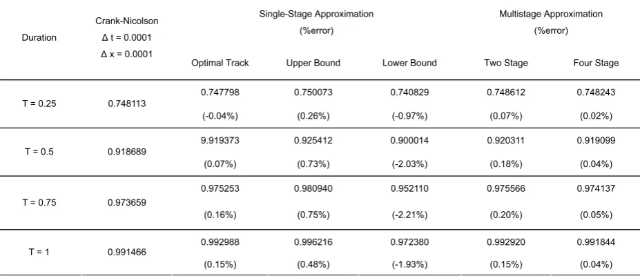
Table 2. Comparison of estimates and bounds of the first passage time distribution function (FPTDF) with the (numerically) exact results by CN method. Percentage error is defined as (estimate or bound – CN result)/ CN result × 100 %. Number of images summed: n= -2 to n =2. Input parameters are: ț = 1, ȝ =0.1, ı = 0.2, r = 0, Su= 110, SL= 90, Sm= 100 and S = 105.
Single-Stage Approximation
(%error)
Multistage Approximation
(%error) Duration
Crank-Nicolson
ǻ t = 0.0001
ǻ x = 0.0001
Optimal Track Upper Bound Lower Bound Two Stage Four Stage
0.747798 0.750073 0.740829 0.748612 0.748243 T = 0.25 0.748113
(-0.04%) (0.26%) (-0.97%) (0.07%) (0.02%)
9.919373 0.925412 0.900014 0.920311 0.919099 T = 0.5 0.918689
(0.07%) (0.73%) (-2.03%) (0.18%) (0.04%)
0.975253 0.980940 0.952110 0.975566 0.974137 T = 0.75 0.973659
(0.16%) (0.75%) (-2.21%) (0.20%) (0.05%)
0.992988 0.996216 0.972380 0.992920 0.991844 T = 1 0.991466
[image:6.595.62.526.510.710.2]