Discriminative Sentence Compression with Soft Syntactic Evidence
Ryan McDonald
Department of Computer and Information Science University of Pennsylvania
Philadelphia, PA 19104 [email protected]
Abstract
We present a model for sentence com-pression that uses a discriminative large-margin learning framework coupled with a novel feature set defined on compressed bigrams as well as deep syntactic repre-sentations provided by auxiliary depen-dency and phrase-structure parsers. The parsers are trained out-of-domain and con-tain a significant amount of noise. We ar-gue that the discriminative nature of the learning algorithm allows the model to learn weights relative to any noise in the feature set to optimize compression ac-curacy directly. This differs from cur-rent state-of-the-art models (Knight and Marcu, 2000) that treat noisy parse trees, for both compressed and uncompressed sentences, as gold standard when calculat-ing model parameters.
1 Introduction
The ability to compress sentences grammatically with minimal information loss is an important problem in text summarization. Most summariza-tion systems are evaluated on the amount of rele-vant information retained as well as their compres-sion rate. Thus, returning highly compressed, yet informative, sentences allows summarization sys-tems to return larger sets of sentences and increase the overall amount of information extracted.
We focus on the particular instantiation of sen-tence compression when the goal is to produce the compressed version solely by removing words or phrases from the original, which is the most com-mon setting in the literature (Knight and Marcu, 2000; Riezler et al., 2003; Turner and Charniak,
2005). In this framework, the goal is to find the shortest substring of the original sentence that con-veys the most important aspects of the meaning. We will work in a supervised learning setting and assume as input a training set T=(xt,yt)|T |t=1 of original sentences xt and their compressions yt.
We use the Ziff-Davis corpus, which is a set of 1087 pairs of sentence/compression pairs. Fur-thermore, we use the same 32 testing examples from Knight and Marcu (2000) and the rest for training, except that we hold out 20 sentences for the purpose of development. A handful of sen-tences occur twice but with different compres-sions. We randomly select a single compression for each unique sentence in order to create an un-ambiguous training set. Examples from this data set are given in Figure 1.
Formally, sentence compression aims to shorten a sentence x = x1. . . xn into a substring y = y1. . . ym, whereyi ∈ {x1, . . . , xn}. We define
the function I(yi) ∈ {1, . . . , n} that maps word yi in the compression to the index of the word in
the original sentence. Finally we include the con-straint I(yi) < I(yi+1), which forces each word inxto occur at most once in the compression y.
Compressions are evaluated on three criteria,
1. Grammaticality: Compressed sentences should be grammatical.
2. Importance: How much of the important in-formation is retained from the original.
3. Compression rate: How much compression took place. A compression rate of 65%
means the compressed sentence is 65% the length of the original.
The Reverse Engineer Tool is priced from $8,000 for a single user to $90,000 for a multiuser project site .
The Reverse Engineer Tool is available now and is priced on a site-licensing basis , ranging from $8,000 for a single user to $90,000 for a multiuser project site .
Design recovery tools read existing code and translate it into defi nitions and structured diagrams .
Essentially , design recovery tools read existing code and translate it into the language in which CASE is conversant – defi nitions and structured diagrams .
Figure 1: Two examples of compressed sentences from the Ziff-Davis corpus. The compressed version and the original sentence are given.
compressions, the less likely we are to remove im-portant words or phrases crucial to maintaining grammaticality and the intended meaning.
The paper is organized as follows: Section 2 discusses previous approaches to sentence com-pression. In particular, we discuss the advantages and disadvantages of the models of Knight and Marcu (2000). In Section 3 we present our dis-criminative large-margin model for sentence com-pression, including the learning framework and an efficient decoding algorithm for searching the space of compressions. We also show how to extract a rich feature set that includes surface-level bigram features of the compressed sentence, dropped words and phrases from the original sen-tence, and features over noisy dependency and phrase-structure trees for the original sentence. We argue that this rich feature set allows the model to learn which words and phrases should be dropped and which should remain in the com-pression. Section 4 presents an experimental eval-uation of our model compared to the models of Knight and Marcu (2000) and finally Section 5 discusses some areas of future work.
2 Previous Work
Knight and Marcu (2000) first tackled this prob-lem by presenting a generative noisy-channel model and a discriminative tree-to-tree decision tree model. The noisy-channel model defines the problem as finding the compressed sentence with maximum conditional probability
y= arg max
y
P(y|x) = arg max
y
P(x|y)P(y)
P(y) is the source model, which is a PCFG plus bigram language model. P(x|y) is the channel model, the probability that the long sentence is an expansion of the compressed sentence. To calcu-late the channel model, both the original and com-pressed versions of every sentence in the training set are assigned a phrase-structure tree. Given a tree for a long sentence x and compressed
sen-tence y, the channel probability is the product of
the probability for each transformation required if the tree foryis to expand to the tree forx.
The tree-to-tree decision tree model looks to rewrite the tree forxinto a tree fory. The model
uses a shift-reduce-drop parsing algorithm that starts with the sequence of words inxand the
cor-responding tree. The algorithm then either shifts (considers new words and subtrees forx), reduces
(combines subtrees fromxinto possibly new tree
constructions) or drops (drops words and subtrees fromx) on each step of the algorithm. A decision
tree model is trained on a set of indicative features for each type of action in the parser. These mod-els are then combined in a greedy global search algorithm to find a single compression.
Though both models of Knight and Marcu per-form quite well, they do have their shortcomings. The noisy-channel model uses a source model that is trained on uncompressed sentences, even though the source model is meant to represent the probability of compressed sentences. The channel model requires aligned parse trees for both com-pressed and uncomcom-pressed sentences in the train-ing set in order to calculate probability estimates. These parses are provided from a parsing model trained on out-of-domain data (the WSJ), which can result in parse trees with many mistakes for both the original and compressed versions. This makes alignment difficult and the channel proba-bility estimates unreliable as a result. On the other hand, the decision tree model does not rely on the trees to align and instead simply learns a tree-to-tree transformation model to compress sentences. The primary problem with this model is that most of the model features encode properties related to including or dropping constituents from the tree with no encoding of bigram or trigram surface fea-tures to promote grammaticality. As a result, the model will sometimes return very short and un-grammatical compressions.
ideally, parse trees should be treated solely as a source of evidence when making compression de-cisions to be balanced with other evidence such as that provided by the words themselves.
Recently Turner and Charniak (2005) presented supervised and semi-supervised versions of the Knight and Marcu noisy-channel model. The re-sulting systems typically return informative and grammatical sentences, however, they do so at the cost of compression rate. Riezler et al. (2003) present a discriminative sentence compressor over the output of an LFG parser that is a packed rep-resentation of possible compressions. Though this model is highly likely to return grammatical com-pressions, it required the training data be human annotated with syntactic trees.
3 Discriminative Sentence Compression
For the rest of the paper we use x = x1. . . xn
to indicate an uncompressed sentence and y = y1. . . yma compressed version ofx, i.e., eachyj
indicates the position inx of thejth word in the
compression. We always pad the sentence with dummy start and end words, x1 = -START- and
xn = -END-, which are always included in the
compressed version (i.e.y1 =x1andym =xn).
In this section we described a discriminative on-line learning approach to sentence compression, the core of which is a decoding algorithm that searches the entire space of compressions. Let the score of a compressionyfor a sentencexas
s(x,y)
In particular, we are going to factor this score us-ing a first-order Markov assumption on the words in thecompressedsentence
s(x,y) = |y| X
j=2
s(x, I(yj−1), I(yj))
Finally, we define the score function to be the dot product between a high dimensional feature repre-sentation and a corresponding weight vector
s(x,y) = |y| X
j=2
w·f(x, I(yj−1), I(yj))
Note that this factorization will allow us to define features over two adjacent words in the compres-sion as well as the words in-between that were dropped from the original sentence to create the
compression. We will show in Section 3.2 how this factorization also allows us to include features on dropped phrases and subtrees from both a de-pendency and a phrase-structure parse of the orig-inal sentence. Note that these features are meant to capture the same information in both the source and channel models of Knight and Marcu (2000). However, here they are merely treated as evidence for the discriminative learner, which will set the weight of each feature relative to the other (pos-sibly overlapping) features to optimize the models accuracy on the observed data.
3.1 Decoding
We define a dynamic programming table C[i]
which represents the highest score for any com-pression that ends at wordxi for sentencex. We
define a recurrence as follows
C[1] = 0.0
C[i] = maxj<iC[j] +s(x, j, i)fori >1
It is easy to show thatC[n]represents the score of the best compression for sentencex(whose length
is n) under the first-order score factorization we made. We can show this by induction. If we as-sume thatC[j]is the highest scoring compression that ends at wordxj, for allj < i, thenC[i]must
also be the highest scoring compression ending at word xi since it represents the max combination
over all high scoring shorter compressions plus the score of extending the compression to the cur-rent word. Thus, sincexnis by definition in every
compressed version ofx(see above), then it must
be the case that C[n]stores the score of the best compression. This table can be filled inO(n2
). This algorithm is really an extension of Viterbi to the case when scores factor over dynamic sub-strings of the text (Sarawagi and Cohen, 2004; McDonald et al., 2005a). As such, we can use back-pointers to reconstruct the highest scoring compression as well as k-best decoding algo-rithms.
this is rarely seen in the training data. In fact, it turns out that our learned compressions have a compression rate very similar to the gold standard. That said, there are some instances when a static compression rate is preferred. A user may specif-ically want a 25% compression rate for all sen-tences. This is not a problem for our decoding algorithm. We simply augment the dynamic pro-gramming table and calculateC[i][r], which is the score of the best compression of lengthrthat ends at wordxi. This table can be filled in as follows
C[1][1] = 0.0
C[1][r] =−∞forr >1
C[i][r] = maxj<iC[j][r−1] +s(x, j, i)fori >1
Thus, if we require a specific compression rate, we simple determine the number of wordsr that sat-isfy this rate and calculateC[n][r]. The new com-plexity isO(n2r).
3.2 Features
So far we have defined the score of a compres-sion as well as a decoding algorithm that searches the entire space of compressions to find the one with highest score. This all relies on a score fac-torization over adjacent words in the compression,
s(x, I(yj−1), I(yj)) = w·f(x, I(yj−1), I(yj)).
In Section 3.3 we describe an online large-margin method for learning w. Here we present the fea-ture representation f(x, I(yj−1), I(yj))for a pair
of adjacent words in the compression. These fea-tures were tuned on a development data set.
3.2.1 Word/POS Features
The first set of features are over adjacent words
yj−1 and yj in the compression. These include
the part-of-speech (POS) bigrams for the pair, the POS of each word individually, and the POS con-text (bigram and trigram) of the most recent word being added to the compression, yj. These
fea-tures are meant to indicate likely words to in-clude in the compression as well as some level of grammaticality, e.g., the adjacent POS features “JJ&VB” would get a low weight since we rarely see an adjective followed by a verb. We also add a feature indicating ifyj−1andyj were actually
ad-jacent in the original sentence or not and we con-join this feature with the above POS features. Note that we have not included any lexical features. We found during experiments on the development data that lexical information was too sparse and led to overfitting, so we rarely include such features. In-stead we rely on the accuracy of POS tags to
pro-vide enough epro-vidence.
Next we added features over every dropped word in the original sentence betweenyj−1andyj,
if there were any. These include the POS of each dropped word, the POS of the dropped words con-joined with the POS ofyj−1andyj. If the dropped
word is a verb, we add a feature indicating the ac-tual verb (this is for common verbs like “is”, which are typically in compressions). Finally we add the POS context (bigram and trigram) of each dropped word. These features represent common charac-teristics of words that can or should be dropped from the original sentence in the compressed ver-sion (e.g. adjectives and adverbs). We also add a feature indicating whether the dropped word is a negation (e.g., not, never, etc.).
We also have a set of features to represent brackets in the text, which are common in the data set. The first measures if all the dropped words betweenyj−1andyjhave a mismatched or
incon-sistent bracketing. The second measures if the left and right-most dropped words are themselves both brackets. These features come in handy for ex-amples like,The Associated Press ( AP ) reported the story, where the compressed version is The Associated Press reported the story. Information within brackets is often redundant.
3.2.2 Deep Syntactic Features
The previous set of features are meant to en-code common POS contexts that are commonly re-tained or dropped from the original sentence dur-ing compression. However, they do so without a larger picture of the function of each word in the sentence. For instance, dropping verbs is not that uncommon - a relative clause for instance may be dropped during compression. However, dropping the main verb in the sentence is uncommon, since that verb and its arguments typically encode most of the information being conveyed.
An obvious solution to this problem is to in-clude features over a deep syntactic analysis of the sentence. To do this we parse every sentence twice, once with a dependency parser (McDon-ald et al., 2005b) and once with a phrase-structure parser (Charniak, 2000). These parsers have been trained out-of-domain on the Penn WSJ Treebank and as a result contain noise. However, we are merely going to use them as an additional source of features. We call this soft syntactic evidence
root0
saw2
on4 after6
Mary1 Ralph3 Tuesday5 lunch7
S
VP
PP PP
NP NP NP NP
NNP VBD NNP IN NNP IN NN
[image:5.595.75.523.61.151.2]Mary1 saw2 Ralph3 on4 Tuesday5 after6 lunch7
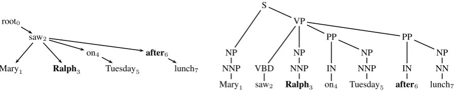
Figure 2: An example dependency tree from the McDonald et al. (2005b) parser and phrase structure tree from the Charniak (2000) parser. In this example we want to add features from the trees for the case whenRalphandafterbecome adjacent in the compression, i.e., we are dropping the phraseon Tuesday.
or against particular compressions. The learning algorithm will set the feature weight accordingly depending on each features discriminative power. It is not unique to use soft syntactic features in this way, as it has been done for many problems in language processing. However, we stress this aspect of our model due to the history of compres-sion systems using syntax to provide hard struc-tural constraints on the output.
Lets consider the sentencex=Mary saw Ralph
on Tuesday after lunch, with corresponding parses given in Figure 2. In particular, lets consider the feature representation f(x,3,6). That is, the
fea-ture representation of makingRalphandafter ad-jacent in the compression and dropping the prepo-sitional phraseon Tuesday. The first set of features we consider are over dependency trees. For every dropped word we add a feature indicating the POS of the words parent in the tree. For example, if the dropped words parent isroot, then it typically means it is the main verb of the sentence and un-likely to be dropped. We also add a conjunction feature of the POS tag of the word being dropped and the POS of its parent as well as a feature in-dicating for each word being dropped whether it is a leaf node in the tree. We also add the same features for the two adjacent words, but indicating that they are part of the compression.
For the phrase-structure features we find every node in the tree that subsumes a piece of dropped text and is not a child of a similar node. In this case the PP governing on Tuesday. We then add fea-tures indicating the context from which this node was dropped. For example we add a feature spec-ifying that a PP was dropped which was the child of a VP. We also add a feature indicating that a PP was dropped which was the left sibling of another PP, etc. Ideally, for each production in the tree we would like to add a feature indicating every node that was dropped, e.g. “VP→VBD NP PP PP⇒ VP→VBD NP PP”. However, we cannot
neces-sarily calculate this feature since the extent of the production might be well beyond the local context of first-order feature factorization. Furthermore, since the training set is so small, these features are likely to be observed very few times.
3.2.3 Feature Set Summary
In this section we have described a rich feature set over adjacent words in the compressed sen-tence, dropped words and phrases from the origi-nal sentence, and properties of deep syntactic trees of the original sentence. Note that these features in many ways mimic the information already present in the noisy-channel and decision-tree models of Knight and Marcu (2000). Our bigram features encode properties that indicate both good and bad words to be adjacent in the compressed sentence. This is similar in purpose to the source model from the noisy-channel system. However, in that sys-tem, the source model is trained on uncompressed sentences and thus is not as representative of likely bigram features for compressed sentences, which is really what we desire.
calculating probability estimates.
An important distinction we should make is the notion of supported versus unsupported features (Sha and Pereira, 2003). Supported features are those that are on for the gold standard compres-sions in the training. For instance, the bigram fea-ture “NN&VB” will be supported since there is most likely a compression that contains a adjacent noun and verb. However, the feature “JJ&VB” will not be supported since an adjacent adjective and verb most likely will not be observed in any valid compression. Our model includes all fea-tures, including those that are unsupported. The advantage of this is that the model can learn nega-tive weights for features that are indicanega-tive of bad compressions. This is not difficult to do since most features are POS based and the feature set size even with all these features is only 78,923.
3.3 Learning
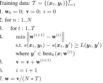
Having defined a feature encoding and decod-ing algorithm, the last step is to learn the fea-ture weights w. We do this using the Margin Infused Relaxed Algorithm (MIRA), which is a discriminative large-margin online learning tech-nique shown in Figure 3 (Crammer and Singer, 2003). On each iteration, MIRA considers a single instance from the training set(xt,yt)and updates
the weights so that the score of the correct com-pression, yt, is greater than the score of all other
compressions by a margin proportional to their loss. Many weight vectors will satisfy these con-straints so we pick the one with minimum change from the previous setting. We define the loss to be the number of words falsely retained or dropped in the incorrect compression relative to the correct one. For instance, if the correct compression of the sentence in Figure 2 isMary saw Ralph, then the compression Mary saw after lunch would have a loss of 3 since it incorrectly left out one word and included two others.
Of course, for a sentence there are exponentially many possible compressions, which means that this optimization will have exponentially many constraints. We follow the method of McDon-ald et al. (2005b) and create constraints only on the k compressions that currently have the high-est score, bhigh-estk(x;w). This can easily be
calcu-lated by extending the decoding algorithm with standard Viterbik-best techniques. On the devel-opment data, we found that k = 10provided the
Training data:T ={(xt,yt)}Tt=1 1.w0= 0; v= 0; i= 0 2. forn: 1..N
3. fort: 1..T
4. min‚‚ ‚w
(i+1)−w(i)‚‚ ‚
s.t.s(xt,yt)−s(xt,y0)≥L(yt,y0)
wherey0∈bestk(x;w(i))
5. v=v+w(i+1) 6. i=i+ 1
[image:6.595.309.475.63.197.2]7.w=v/(N∗T)
Figure 3: MIRA learning algorithm as presented by McDonald et al. (2005b).
best performance, though varyingkdid not have a major impact overall. Furthermore we found that after only 3-5 training epochs performance on the development data was maximized.
The final weight vector is the average of all weight vectors throughout training. Averaging has been shown to reduce overfitting (Collins, 2002) as well as reliance on the order of the examples during training. We found it to be particularly im-portant for this data set.
4 Experiments
We use the same experimental methodology as Knight and Marcu (2000). We provide every com-pression to four judges and ask them to evaluate each one for grammaticality and importance on a scale from 1 to 5. For each of the 32 sentences in our test set we ask the judges to evaluate three sys-tems: human annotated, the decision tree model of Knight and Marcu (2000) and our system. The judges were told all three compressions were au-tomatically generated and the order in which they were presented was randomly chosen for each sen-tence. We compared our system to the decision tree model of Knight and Marcu instead of the noisy-channel model since both performed nearly as well in their evaluation, and the compression rate of the decision tree model is nearer to our sys-tem (around 57-58%). The noisy-channel model typically returned longer compressions.
Results are shown in Table 1. We present the av-erage score over all judges as well as the standard deviation. The evaluation for the decision tree sys-tem of Knight and Marcu is strikingly similar to the original evaluation in their work. This provides strong evidence that the evaluation criteria in both cases were very similar.
com-Compression Rate Grammaticality Importance
[image:7.595.142.464.62.109.2]Human 53.3% 4.96±0.2 3.91±1.0 Decision-Tree (K&M2000) 57.2% 4.30±1.4 3.60±1.3 This work 58.1% 4.61±0.8 4.03±1.0
Table 1: Compression results.
pressions rates, with humans preferring to com-press a little more aggressively. Not surprisingly, the human compressions are practically all gram-matical. A quick scan of the evaluations shows that the few ungrammatical human compressions were for sentences that were not really gram-matical in the first place. Of greater interest is that the compressions of our system are typically more grammatical than the decision tree model of Knight and Marcu.
When looking at importance, we see that our system actually does the best – even better than humans. The most likely reason for this is that our model returns longer sentences and is thus less likely to prune away important information. For example, consider the sentence
The chemical etching process used for glare protection is effective and will help if your office has the fluorescent-light
overkill that’s typical in offices
The human compression was Glare protection is effective, whereas our model compressed the sen-tence to The chemical etching process used for glare protection is effective.
A primary reason that our model does better than the decision tree model of Knight and Marcu is that on a handful of sentences, the decision tree compressions were a single word or noun-phrase. For such sentences the evaluators typically rated the compression a 1 for both grammaticality and importance. In contrast, our model never failed in such drastic ways and always output something reasonable. This is quantified in the standard de-viation of the two systems.
Though these results are promising, more large scale experiments are required to really ascer-tain the significance of the performance increase. Ideally we could sample multiple training/testing splits and use all sentences in the data set to eval-uate the systems. However, since these systems require human evaluation we did not have the time or the resources to conduct these experiments.
4.1 Some Examples
Here we aim to give the reader a flavor of some common outputs from the different models. Three examples are given in Table 4.1. The first shows
two properties. First of all, the decision tree model completely breaks and just returns a sin-gle noun-phrase. Our system performs well, how-ever it leaves out the complementizer of the rela-tive clause. This actually occurred in a few exam-ples and appears to be the most common problem of our model. A post-processing rule should elim-inate this.
The second example displays a case in which our system and the human system are grammati-cal, but the removal of a prepositional phrase hurts the resulting meaning of the sentence. In fact, without the knowledge that the sentence is refer-ring to broadband, the compressions are mean-ingless. This appears to be a harder problem – determining which prepositional phrases can be dropped and which cannot.
The final, and more interesting, example presents two very different compressions by the human and our automatic system. Here, the hu-man kept the relative clause relating what lan-guages the source code is available in, but dropped the main verb phrase of the sentence. Our model preferred to retain the main verb phrase and drop the relative clause. This is most likely due to the fact that dropping the main verb phrase of a sen-tence is much less likely in the training data than dropping a relative clause. Two out of four eval-uators preferred the compression returned by our system and the other two rated them equal.
5 Discussion
In this paper we have described a new system for sentence compression. This system uses discrim-inative large-margin learning techniques coupled with a decoding algorithm that searches the space of all compressions. In addition we defined a rich feature set of bigrams in the compression and dropped words and phrases from the original sen-tence. The model also incorporates soft syntactic evidence in the form of features over dependency and phrase-structure trees for each sentence.
compres-Full Sentence The fi rst new product , ATF Protype , is a line of digital postscript typefaces that will be sold in packages of up to six fonts . Human ATF Protype is a line of digital postscript typefaces that will be sold in packages of up to six fonts .
Decision Tree The fi rst new product .
This work ATF Protype is a line of digital postscript typefaces will be sold in packages of up to six fonts .
Full Sentence Finally , another advantage of broadband is distance . Human Another advantage is distance .
Decision Tree Another advantage of broadband is distance . This work Another advantage is distance .
Full Sentence The source code , which is available for C , Fortran , ADA and VHDL , can be compiled and executed on the same system or ported to other target platforms .
Human The source code is available for C , Fortran , ADA and VHDL . Decision Tree The source code is available for C .
This work The source code can be compiled and executed on the same system or ported to other target platforms .
Table 2: Example compressions for the evaluation data.
sion accuracy during training, both of which have been shown to be beneficial for other problems. Furthermore, the system does not rely on the syn-tactic parses of the sentences to calculate probabil-ity estimates. Instead, this information is incorpo-rated as just another form of evidence to be consid-ered during training. This is advantageous because these parses are trained on out-of-domain data and often contain a significant amount of noise.
A fundamental flaw with all sentence compres-sion systems is that model parameters are set with the assumption that there is a single correct answer for each sentence. Of course, like most compres-sion and translation tasks, this is not true, consider, TapeWare , which supports DOS and NetWare 286 , is a
value-added process that lets you directly connect the
QA150-EXAT to a file server and issue a command from any workstation to back up the server
The human annotated compression is, TapeWare supports DOS and NetWare 286. However, an-other completely valid compression might be,
TapeWare lets you connect the QA150-EXAT to a fi le server. These two compressions overlap by a single word.
Our learning algorithm may unnecessarily lower the score of some perfectly valid compres-sions just because they were not the exact com-pression chosen by the human annotator. A pos-sible direction of research is to investigate multi-label learning techniques for structured data (Mc-Donald et al., 2005a) that learn a scoring function separating a set of valid answers from all invalid answers. Thus if a sentence has multiple valid compressions we can learn to score each valid one higher than all invalid compressions during train-ing to avoid this problem.
Acknowledgments
The author would like to thank Daniel Marcu for providing the data as well as the output of his
and Kevin Knight’s systems. Thanks also to Hal Daum´e and Fernando Pereira for useful discus-sions. Finally, the author thanks the four review-ers for evaluating the compressed sentences. This work was supported by NSF ITR grants 0205448 and 0428193.
References
E. Charniak. 2000. A maximum-entropy-inspired
parser. InProc. NAACL.
M. Collins. 2002. Discriminative training methods for hidden Markov models: Theory and experiments
with perceptron algorithms. InProc. EMNLP.
K. Crammer and Y. Singer. 2003. Ultraconservative
online algorithms for multiclass problems.JMLR.
K. Knight and D. Marcu. 2000. Statistical-based sum-marization - step one: Sentence compression. In
Proc. AAAI 2000.
R. McDonald, K. Crammer, and F. Pereira. 2005a. Flexible text segmentation with structured
multil-abel classifi cation. InProc. HLT-EMNLP.
R. McDonald, K. Crammer, and F. Pereira. 2005b. On-line large-margin training of dependency parsers. In
Proc. ACL.
S. Riezler, T. H. King, R. Crouch, and A. Zaenen. 2003. Statistical sentence condensation using ambi-guity packing and stochastic disambiguation
meth-ods for lexical-functional grammar. In Proc.
HLT-NAACL.
S. Sarawagi and W. Cohen. 2004. Semi-Markov con-ditional random fi elds for information extraction. In
Proc. NIPS.
F. Sha and F. Pereira. 2003. Shallow parsing with
con-ditional random fi elds. InProc. HLT-NAACL, pages
213–220.
J. Turner and E. Charniak. 2005. Supervised and un-supervised learning for sentence compression. In