An Automated Model Generation Approach for
High Level Modelling
Likun Xia, Ian M. Bell, and Antony J. Wilkinson
Abstract—Over the last few years automated model generation has become an increasingly important component of methodologies for verification of large, complex mix-signal SoCs (system-on-chips) and SiPs (system-in-packages). In this paper a novel approach termed Multiple Model Generation System using Delta operator (MMGSD) is developed for extracting either single-input single-output (SISO) or multiple-input single-output (MISO) macromodels from a SPICE netlist. This model generation process detects nonlinearity through variations in output error. Examples of the application of MMGSD are presented for simple two-input systems incorporating a two-stage CMOS operational amplifier (op amp). We demonstrate the generated models are able to model various circuits with good accuracy.
Keywords—Automated Model Generation, Analogue Modelling
I. INTRODUCTION
During the last few years, high level modelling (HLM) techniques have been proposed for modern complex analogue and mixed-mode system design. These models can be obtained in two ways: manual and automatic. This paper focuses on the latter. There are several broad methodologies for automated model generation (AMG), which have been discussed and utilized in many papers. Initially a designer decides the model structure, which includes linear time-invariant (LTI), linear time-variant (LTV), nonlinear time-invariant and nonlinear time-variant. An estimation algorithm is then required in order to obtain parameters for these models. This algorithm may be regression [7],[8], lookup tables [1], radial basis functions (RBF) [2], and artificial neural networks (ANN) [3],[4] and its derivations such as fuzzy logic (FL) [5] and neural-fuzzy network (NF) [6]. They may be categorized into the black-box or grey-box approach. The grey-box is used when some knowledge of the internal structure of the model is known. The white-box is also one of these approaches, but structures and parameters of models are already known. Automated model generation can be realized with these approaches.
Unfortunately, some of the models generated are of high order (e.g., [9]–[11]) resulting in excessive complexity, so model order reduction (MOD) techniques are required [12]. Many papers have summarized these techniques based on MOR (e.g., [13]): LTI MOR [14], LTV MOR [15],[16] and
Likun Xia, Department of Engineering, The University of Hull, Hull, UK (Tel: +44 (0)1482 465384; email: [email protected])
Ian M. Bell, Department of Engineering, The University of Hull, Hull, UK ([email protected])
Antony J. Wilkinson, Department of Engineering, The University of Hull, Hull, UK ([email protected])
weakly nonlinear methods including polynomialbased NORM [17],[18] and piecewise approximation method -trajectory piecewise linear (TPWL) [19], piecewise polynomial (PWP) [20]. PWP is further employed [21],[22] to capture different loading effects, simultaneous switching noise (SSN), crosstalk noise and so on, faster modelling speed is achieved, but multiple training data have to be required [22] to cover various regions.
A previous work termed MMGS (multiple model generation system) was developed based on training data from pseudorandom binary sequence generator (PRBSG) [23]. This system generates new models by observing variation in output error voltage. The advantage is that the estimated signal can be adjusted recursively in time to handle nonlinearity. However, this approach is based on discrete-time operation, so its parameters have a strong dependence on the sampling interval, incurring disadvantages such as aliasing and slow simulation speed.
For straightforward system simulation relatively simple models may be adequate, must most published approaches have not proven their models work well under system fault simulation. Faulty behaviour may force (non-faulty) subsystems into highly nonlinear regions of operation, which may not be covered by their models.
In this paper we developed a novel approach named multiple model generation system using delta operator (MMGSD) for generating either single-input single-output (SISO) or multiple-input single-output (MISO) macromodels. It is similar to MMGS except that we employ delta transform instead of discrete-time transform, i.e., this model generation process still detects nonlinearity through variations in output error. By using the delta operator the coefficients produced relate to physical quantities as in the continuous-time domain model and are less susceptible to the choice of sampling interval provided it is chosen appropriately [24].
II. OVERVIEW OF MMGSD
start
Pre-measuring for the input data
Add a model
Post-analysis Estimator
yes
no
end
New model needed?
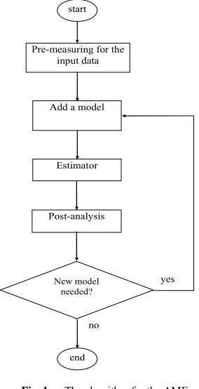
Fig. 1 The algorithm for the AME system Estimator is based on modified recursively maximum likelihood (RML) estimation [8], which is an extension of the recursive least square (RLS) estimate using delta transformed signal data. The model structure is related to the Laplace transfer function of process as follows. Initially a continuous time transfer function is considered in (1).
0 1
1
0 1
1 0
)
(
s
a
s
a
s
s
b
s
b
s
b
s
G
m m
m
n n
n
(1)When sampling interval is sufficiently short, the continuous time transfer functionG(s) is equal to the delta
transfer functionG(δ) [7] shown in (2).
0 1
1
0 1
1 0
)
(
)
(
)
(
m m
m
n n
n
a
a
b
b
b
t
u
t
y
G
(2)After arranging this equation, (3) is obtained:
)
(
)
(
)
(
)
(
)
(
0
1 1
t
u
b
b
t
y
a
a
t
y
n n
m m
m
(3)
It is known that error is related to the quality of estimation, i.e., a smaller error indicates that a better estimated signal has been achieved. Thus the variation in output error against the input amplitude is analyzed in the MMGSD to decide if a new model needs to be generated. In RML there are two error parameters: the innovation error
epsiand residual errorepsilon, both involve the difference
between the original signal and the estimated one. However,
epsiis not only related to the value at current time but also
the one at previous time, which is difficult to observe. Therefore,epsilonis selected for observing its variation.
Initially the number of intervals on the input voltage is set up to determine where the models should be. The decision to add a new model on one of the intervals is based on three equations shown in (4):
nge criticalRa
dex smallestin e
mediumRang e
mediumRang criteria
l lowInterva al
highInterv nge
criticalRa
l lowInterva al
highInterv e
mediumRang
)] (
[
2 / ) (
2 / ) (
where the medium range mediumRange is the half of
difference between the maximum amplitude of error
maxInterval and the minimum amplitude of error
minIntervalin the same interval;criticalRangeis equivalent
to the half of summation tomaxIntervaland minInterval;
the variable criteria is the difference between the mediumRange andcriticalRangeat the same interval and
then subtracts mediumRange; smallestindex is the index
appointing to the interval where minimum range ofepsilon
is.
A new model is required in an interval whencriteriais
greater or equal to zero, otherwise no action is taken. Only one model is created per iteration (figure 1), which is necessary because the shape of the error changes when a model is added. This process is complete when the number of models does not increase any more.
The two-stage CMOS operational amplifier (op amp) shown in Fig. 2 is used to illustrate our methodology. The input state is realized as a CMOS differential amplifier using p-channel MOSFETs. The differential amplifier is biased with the current mirror M13&M14. Three NMOS diodes (M4, M5 and M6) are used to keep the gate to source voltage of the current mirror small (VGS = -1.175V). The output stage (M7 and M10) is a simple CMOS push-pull inverter.
M4
M5
M6
M13 M14
M11 M12
M8 M9
C
C
M10
M7 Vdd
Vss
In- In+
Out
2
1 4
4
12
12 11
5
8
3 0
6
9
IEE Iref
Fig. 2 Schematic of the two-stage CMOS operational amplifier The input signal used to produce training data for the estimator is a 93.34 Hz, 0.25V triangle waveform with a 0.04V and a time interval of 10us pseudorandom binary
sequence (PRBS) superimposed on it. The similar signal but with different amplitude and frequency is applied to the non-inverting input.
During simulation (estimation) some quantities in the system need to be either deltarised or undeltarised, for example, epsilon in the AME and AMP is already
[image:2.595.93.235.51.328.2] [image:2.595.328.541.482.620.2]MMGSD: the Deltarise function and Undeltarise function. The former is to generate derivative vectors based on original vectors. The undeltarise function requires original data during the estimation. These two functions are used in different places in the MMGSD.
A. The Deltarise Function
The deltarise function is used to achieve deltarised value based on the Delta operator seen in (5), where delta (δ) is related to both the present and future values, Ts is the
sampling rate, q is the forward shift operator used to
describe discrete models, which is shown in (6).
dt d T q
s
1
(5)
qx
k
x
k1 (6) The equivalent form of (6) is obtained in (7), the relationship betweenδandqis a simple linear function, soδ
can offer the same flexibility in the modelling of discrete-time systems asqdoes.
dt dx T
kT x T kT x T
x x x
s
s s
s
s k k
k
1 ( ) ( )
(7)The use of delta operator and its relationship is illustrated in the following example. It is a discrete-time model but only output vectors are displayed in (8). Initially each vector except the last one is subtracted from the one next to it, and is then divided byTs, so deltarised value is obtained, as seen
in (9). The same procedure for (9) is then repeated in order to achieve fully deltarised vectors seen in (10).
y(t) y(t-1) y(t-2) y(t-3) (8)
δy(t-1)δy(t-2) δy(t-3) (9)
δ2y(t-3)δ1y(t-3)δ0y(t-3) (10)
B. The Undeltarise Function
This function is based on (5) but with modification, that is, q = δTs+1, in order to model at the current time. An
example is also used to demonstrate this reverse algorithm. It is a model in delta transform, but only output vectors are displayed in (11). Firstly each vector, except for last one, is multiplied byTsin (12), because it is already undeltarised,
and then adds ones in (13), so undeltarised vectors are obtained in (14), i.e.,y(t-2) is obtained. It is noticed that (13)
is similar to (11) without the highest order vectorδ3y(t-3).
δ3y(t-3) δ2y(t-3) δ1y(t-3) δ0y(t-3) (11) Tsδ3y(t-3) Tsδ2y(t-3) Tsδ1y(t-3) (12)
+ + +
δ2y(t-3) δ1y(t-3) δ0y(t-3) (13)
|| || ||
δ2y(t-2) δ1y(t-2) y(t-2) (14)
The same process is then implemented to achievey(t-1)
ory(t), respectively.
III. MULTIPLE MODEL CONVERSION SYSTEM The multiple model conversion system (MMCS) is implemented in the MATLAB environment. The conversion is from MATLAB to VHDL-AMS and the format of the behavioural model is based on a behavioural model illustrated in Fig. 3.
- ro
ri
+
gnd
Vin MMGSD
out
Voffin
Voffout
Fig. 3 The structure of the behavioural op amp model It comprises two resistors
r
i andr
othat represent theinput impedance and output impedance, respectively,voffin
andvoffoutmodel input and output offsets, respectively. The
models from MMGSD are implemented using a voltage controlled voltage source (VCVS), i.e.,Vo f(Vin) . Output voltages are selected simultaneously depending on the input range to achieve the bumpless transfer. This model selection algorithm is described in Fig. 4.
Ifthe input signal is within the range for the first model
The first model is selected
Else ifthe input signal is within the range for the second model
The second model is selected . . .
Elsethe input signal is not included in these ranges
Either the first or the last model is selected
Fig. 4 The algorithm for model selection IV. EXPERIMENTAL RESULTS
A. System Test
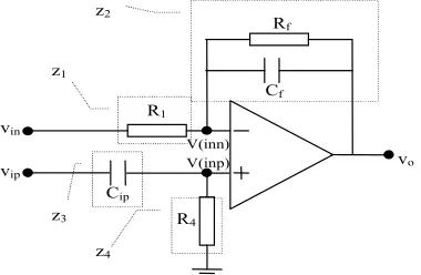
In this section we demonstrate that the MMGSD is able to detect a single model. A linear lead-lag circuit is employed with a high-pass filter and low-pass filter with frequencies of 1kHz and 10Hz seen in Fig. 5, whereR1=
1kΩ,Rf= 10kΩ,Cf = 0.15915uF, R4= 10kΩand Cip =
15.915nF.
R1
R4
vo
vin
vip
Rf
Cf
Cip
V(inn) V(inp)
z2
z3
z4
z1
[image:3.595.323.531.140.243.2] [image:3.595.330.520.629.753.2] [image:3.595.77.246.645.722.2]Its transfer function is shown in (15): ip ip f f ip f f f in f f f o v s R C R s C R R s R C R R s C R R v R s C R R R v ) 1 ( ) ( ) ( ) ( 4 1 1 4 1 1 1 1 (15)
The system was analysed using the system identification toolbox in MATLAB to generate the polynomial based model seen in Fig. 6 with the same PRBS signals as above, where B1 and B2 are coefficients for inputs, F1 and F2 represent the output.
Continuous-time IDPOLY model: y(t) = [B(s)/F(s)]u(t) + e(t) B1(s) = -62.83 s - 3.948e004
B2(s) = s^2 + 69.12 s F1(s) = s^2 + 634.6 s + 3948 F2(s) = s^2 + 634.6 s + 3948
Fig. 6 Coefficients from the analytical simulation Both input and output data are then stored in a text file. The MMGSD was used to generate a model based on this data, as seen in (16). The output coefficients are very close to F1 and F2 in Fig. 6 and the two input coefficients are very close to B1 and B2.
2 . 3825 3 . 615 ) 16 . 67 ( ) 38252 812 . 62 ( 2 2 s s V s s V s
Vo in ip (16)
This proves that the MMGSD is able to handle various circuits including high-pass and low-pass filters, whereas [23] is only able to handle low-pass filters.
B. Verification on the Multiple Model Generation Approach
In this section we verify that multiple models generated by the MMGSD can achieve the bumpless transfer. Initially we set up three stable models with different poles for the AMP, as shown in (17). Each of them has two input parameters and one offset parameter.
1500 20 250 ) 250 10 ( ) 500 20
( 20 1000
250 ) 250 10 ( ) 500 20
( 20 500
250 ) 250 10 ( ) 500 20 ( 2 3 3 3 3 2 2 2 2 2 2 1 1 1 1 s s V V s V s V s s V V s V s V s s V V s V s V offset ip in o offset ip in o offset ip in o (17)
The same PRBS stimulus as above is used. The intervals used to divide the range of this stimulus for these models are: [-0.25V 0.0V 0.095V 0.25V], the sampling rate Tsis
0.1ms. After simulation both input and output data are stored in a text file. The AME then loads this data to produce the models shown in (18). These coefficients generated are close to ones in (17), although the third model is not as accurate as the others because as the pole value is
gets higher, instability is more likely. This is improved by selecting a smaller value such as 1200 instead of 1500.
1390 43 . 18 3 . 248 ) 239 10 ( ) 5 . 483 20
( 20 1000
01 . 250 ) 250 10 ( ) 500 20
( 20 499.5
249 ) 250 10 ( ) 500 20 ( 2 3 3 3 3 2 2 2 2 2 2 1 1 1 1 s s V V s V s V s s V V s V s V s s V V s V s V offset ip in o offset ip in o offset ip in o (18)
An accurate result is also obtained when the same procedure is implemented but based on four models with different poles. This proves that the MMGSD is able to generate various suitable models.
C. Nonlinearity Modelling
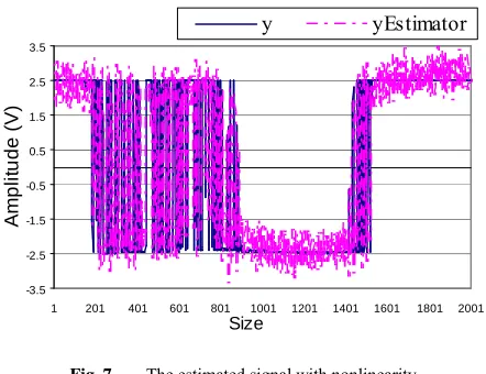
[image:4.595.52.284.50.117.2]In this section the open-loop op amp SPICE netlist from Fig. 2 is modelled using training data which creates strong nonlinearity (into saturation). A new stimulus used is a 2.5V, 83.33Hz triangle waveform with a 0.5V, 100kHz PRBS superimposed on it. A similar signal but with different amplitude and frequency is applied to the non-inverting input. The estimated single yEstimate is
illustrated in Fig. 7 (last 2000 samples). Seven models are generated using the MMGSD. Wherex axis indicates the
number of samples, theyaxis shows the amplitude (V).
-3.5 -2.5 -1.5 -0.5 0.5 1.5 2.5 3.5
1 201 401 601 801 1001 1201 1401 1601 1801 2001 Size A m p li tu d e (V ) y yEstimator
Fig. 7 The estimated signal with nonlinearity
It is seen that yEstimateis able to match the originaly,
even though there is some noise due to the character of delta transform (high sample rate). The difference between two signals is measured using an average difference measurement in (19).
100 _ ) ( ) ( _ 1
peak to peak y N i yP i y dif Average N i where Average_dif is the percentage of average
difference.y(i) -yP(i) is the difference between the original
signal and predicted signal at ith point. N represents the
number of samples. y_peak-to-peak is the peak-to-peak
[image:4.595.313.547.85.172.2] [image:4.595.319.540.394.564.2]average difference is 9.5768% for the simulation described above.
This is improved by employing a system without strong nonlinearity. A differential amplifier with the gain of -2 is employed. The same PRBS as above is connected to the circuit, and the estimated signal is shown in Fig. 8:
0.25 0.35 0.45 0.55 0.65 0.75
1 21 41 61 81 101 121 141 161 181 201
Size
A
m
p
li
tu
d
e
(V
)
y yEstimator
Fig. 8 The estimated signal from a differential amplifier The average difference between the estimated signal
yEstimatorand original signalyis 0.0102%.
D. High Level Modelling
High level modelling (HLM) is implemented based on the behavioural model in Fig. 3. The same models described in section D are converted by the MMCS and then put into this behavioural model. Both transistor level simulation and high level simulation are run in SystemVision.
An inverting amplifier was modelled. The stimulus is a sine waveform with the amplitude of 0.1V and the frequency of 120kHz, and the transient analysis is implemented. Output voltage signals are plotted in Fig. 9.
Fig. 9 The signal from the inverting amplifier
It is seen that the signal from the transistor level simulation (TLS) vout_TLS can be matched by the high
level simulation (HLS) vout_HLM. The cpu time of TLS
and HLS are about 1.891s and 1.672s, respectively. HLS is about 0.22s faster than TLS. Compared with the similar result based on the MMGS [23] speed-up has been achieved.
Secondly a quadratic low-pass filter seen in Fig. 10 was used investigated. It consists of a lossy integrator, an
integrator and an inverting amplifier in series. Global feedback provided by R1 and R5. A low pass filter characteristic (output of op2) and bandpass filter characteristic (output of op1) can be realized with this filter.
op1 op2 op3
in
out
R5
R1
R2 C2
R3 R4
R6
C1 100k
100k 100k 100k
100k 0.01u
0.01u
70.7k
[image:5.595.313.540.116.246.2]1 2 3 4 5
Fig. 10 The quadratic low-pass filter
The transfer function from the input node ‘in’ to the output node ‘out’ is shown in (19).
2 1 5 3
1 1
2
2 1 3 1 2
C C R R C R
s s
C C R R
s
v v
in out
(19)
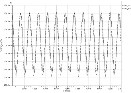
The same behavioural model as above replaces the first operational amplifier (op amp) and the rest of them remain at transistor level. A sine waveform with amplitude 2.5V at 80Hz was used. A transient analysis was performed; output signals from TLSvout_spand HLSvout_mixare plotted in
[image:5.595.56.282.136.298.2]Fig. 11. It is seen that these models are able to model saturation with good accuracy. The total cpu time for HLS is 2.03s, and 1.2s for TLS.
Fig. 11 The output signals from the low-pass filter
A sine waveform with the amplitude of 2.5V at 40Hz is also connected to this circuit. The output signals are plotted in Fig. 12. It is shown that the nonlinearity can be modelled correctly. The total cpu time for the behavioural model is 1.625s, for TLS is 1.2s.
[image:5.595.312.545.483.652.2] [image:5.595.49.279.489.652.2]consuming. The high order of models may reduce the simulation speed, this can be improved by using model order reduction (MOR) approaches.
Fig. 12 The output signals from the low-pass filter V. CONCLUSION AND FUTURE WORK
In this paper the multiple model generation system using Delta operator (MMGSD) is developed for either SISO or MISO models from transistor level SPICE simulations. It is able to converge twice as fast as discrete-time models. We have proved that generated models can achieve bumpless transfer, handle both low-pass and high-pass filters accurately, and model nonlinear behaviours. A multiple model conversion system (MMCS) is developed to convert these models into continuous-time VHDL-AMS behavioural models. High level modelling (HLM) is implemented based on this behavioural model.
Results have shown these models are able to model nonlinear signals with good accuracy. Speed-up may hardly be obtained compared with the transistor level simulation. We are currently investigating model order reduction (MOR) approaches to obtain higher modelling speed. In the future high level fault modelling (HLFM) based on our models will be studied.
VI. REFERENCES
[1] B. Yang and B. MacGaughy, “An Essentially Non-Oscillatory (ENO) High-Order Accurate Adaptive Table Model for Device Modeling”,
Proc. IEEE DAC, 2004.
[2] B. Mutnury, M. Swaminathan, and J. Libous, “Macro-modelling of non-linear I/O drivers using spline functions and finite time difference approximation”, Proc. Electrical Performance of Electronic Packaging, 2003, pp. 273-276.
[3] E. Davalo, P. Naïm, “Neural Networks”,Macmillan Education Ltd.,
1991.
[4] Q, Zhang and K. Gupta, “Neural Networks for RF and Microwave Design”,IEEE Transactions On Microwave Theory And Techniques,
VOL. 51, NO. 4, APRIL 2003.
[5] K.D. Kaehler, “Fuzzy Logic - An Introduction”,
http://www.seattlerobotics.org/encoder/mar98/fuz/fl_part1.html#W HERE%20DID%20FUZZY%20LOGIC%20COME%20FROM?, Available online.
[6] F.J. Uppal and R.J. Patton, “Neuro-fuzzy uncertainty de-coupling: a multiple-model paradigm for fault detection and isolation”,Int. J. Adapt. Control Signal Process, 2005, pp. 281-304.
[7] R.H. Middleton, G.C. Goodwin,Digital Control and Estimation – A Unified Approach, Prentice-Hall, Inc., 1990.
[8] L. Ljung,System Identification-Theory for the User, 2nd Edition,
Prentice-Hall, Inc., 1999.
[9] X. Huang, C.S. Gathercole, and H.A. Mantooth, “Modeling nonlinear dynamics in analog circuits via root localization”,IEEE Trans. CAD,
22(7), July 2003, pp. 895-907.
[10] S.X.-D Tan and C.J.-R Shi, “Efficient DDD-based term generation algorithm for analog circuit behavioral modeling”, Proc. IEEE ASP-DAC, January 2003, pp. 789-794.
[11] Y. Wei and A. Doboli, “Systematic Development of Analog Circuit Structural Macromodels through Behavioral Model Decoupling”,
DAC, June, 2005.
[12] G. Gielen, T. McConaghy, T. Eechelaert, “Performance Space Modeling for Hierarchical Synthesis of Analog Integrated Circuits”,
DAC, June 2005.
[13] J. Roychowdhury, “Automated Macromodel Generation for Electronic Systems”, IEEE Behavioral Modeling and Simulation Workshop, San Jose, CA, Oct. 2003.
[14] L.T. Pillage and R.A. Rohrer, “Asymptotic waveform evaluation for timing analysis”,IEEE Trans. CAD, vol. 9, April 1990, pp. 352-366.
[15] J. Phillips, “Model reduction of time-varying linear systems using approximate multipoint Krylov-subspace projectors”,International Conference on Computer Aided-Design, Santa Clara, California,
November 1998, pp. 96-102.
[16] J. Roychowdhury, “Reduced-Order Modelling of Time-Varying Systems”,IEEE Transactions on circuits and systems-II: Analog and Digital Signal Processing, Vol. 46, No. 10, October 1999.
[17] P. Li and L.T. Pileggi, “NORM: Compact Model Order Reduction of Weakly Nonlinear Systems”,Proceeding of ACM/IEEE DAC, 2003.
[18] P. Li and L.T. Pileggi, “Compact Reduced-order Modeling of Weakly Nonlinear Analog and RF Circuits”,IEEE Transactions on computer-aided design of integrated circuits and systems, vol. 23, No.
2, February 2005.
[19] M. Rewienski and J. White, “A Trajectory Piecewise-Linear Approach to Model-Order Reduction and Fast Simulation of Nonlinear Circuits and Micromachined Devices”, Proceedings IEEE/ACM International Conference on Computer Aided Design,
2001, pp. 252-257.
[20] N. Dong and J. Roychowdhury, “Piecewise Polynomial Nonlinear Model Order Reduction”, Proceedings Design Automation Conference, 2003, pp. 484-489.
[21] N. Dong and J. Roychowdhury, “Automated extraction of broadly applicable nonlinear analog macromodels from SPICE-level descriptions”,CICC, 2004.
[22] N. Dong and J. Roychowdhury, “Automated extraction of Output Buffers for High-Speed Digital Applications”,DAC, 2005.
[23] Likun Xia, I.M. Bell, A.J. Wilkinson, “A Novel Approach for Automated Model Generation”,ISCAS, 2008.