Semi-Supervised Structured Output Learning
based on a Hybrid Generative and Discriminative Approach
Jun Suzuki, Akinori Fujino and Hideki Isozaki
NTT Communication Science Laboratories, NTT Corp. 2-4 Hikaridai, Seika-cho, Soraku-gun, Kyoto, 619-0237 Japan
{jun, a.fujino, isozaki}@cslab.kecl.ntt.co.jp
Abstract
This paper proposes a framework for semi-supervised structured output learning (SOL), specifically for sequence labeling, based on a hybrid generative and discrim-inative approach. We define the objective function of our hybrid model, which is writ-ten in log-linear form, by discriminatively combining discriminative structured predic-tor(s) with generative model(s) that incor-porate unlabeled data. Then, unlabeled data is used in a generative manner to in-crease the sum of the discriminant functions for all outputs during the parameter estima-tion. Experiments on named entity recogni-tion (CoNLL-2003) and syntactic chunking (CoNLL-2000) data show that our hybrid model significantly outperforms the state-of-the-art performance obtained with super-vised SOL methods, such as conditional ran-dom fields (CRFs).
1 Introduction
Structured output learning (SOL) methods, which attempt to optimize an interdependent output space globally, are important methodologies for certain natural language processing (NLP) tasks such as part-of-speech tagging, syntactic chunking (Chunk-ing) and named entity recognition (NER), which are also referred to as sequence labeling tasks. When we consider the nature of these sequence labeling tasks, a semi-supervised approach appears to be more nat-ural and appropriate. This is because the number of features and parameters typically become extremely large, and labeled examples can only sparsely cover the parameter space, even if thousands of labeled
ex-amples are available. In fact, many attempts have re-cently been made to develop semi-supervised SOL methods (Zhu et al., 2003; Li and McCallum, 2005; Altun et al., 2005; Jiao et al., 2006; Brefeld and Scheffer, 2006).
With the generative approach, we can easily in-corporate unlabeled data into probabilistic models with the help of expectation-maximization (EM) al-gorithms (Dempster et al., 1977). For example, the Baum-Welch algorithm is a well-known algorithm for training a hidden Markov model (HMM) of se-quence learning. Generally, with sese-quence learning tasks such as NER and Chunking, we cannot expect to obtain better performance than that obtained us-ing discriminative approaches in supervised learnus-ing settings.
In contrast to the generative approach, with the discriminative approach, it is not obvious how un-labeled training data can be naturally incorporated into a discriminative training criterion. For ex-ample, the effect of unlabeled data will be elimi-nated from the objective function if the unlabeled data is directly used in traditional i.i.d. conditional-probability models. Nevertheless, several attempts have recently been made to incorporate unlabeled data in the discriminative approach. An approach based on pairwise similarities, which encourage nearby data points to have the same class label, has been proposed as a way of incorporating unlabeled data discriminatively (Zhu et al., 2003; Altun et al., 2005; Brefeld and Scheffer, 2006). However, this approach generally requires joint inference over the whole data set for prediction, which is not practi-cal as regards the large data sets used for standard sequence labeling tasks in NLP. Another discrim-inative approach to semi-supervised SOL involves the incorporation of an entropy regularizer
valet and Bengio, 2004). Semi-supervised condi-tional random fields (CRFs) based on a minimum entropy regularizer (SS-CRF-MER) have been pro-posed in (Jiao et al., 2006). With this approach, the parameter is estimated to maximize the likelihood of labeled data and the negative conditional entropy of unlabeled data. Therefore, the structured predictor is trained to separate unlabeled data well under the entropy criterion by parameter estimation.
In contrast to these previous studies, this paper proposes a semi-supervised SOL framework based on a hybrid generative and discriminative approach. A hybrid approach was first proposed in a super-vised learning setting (Raina et al., 2003) for text classification. (Fujino et al., 2005) have developed a semi-supervised approach by discriminatively com-bining a supervised classifier with generative mod-els that incorporate unlabeled data. We extend this framework to the structured output domain, specifi-cally for sequence labeling tasks. Moreover, we re-formalize the objective function to allow the incor-poration of discriminative models (structured pre-dictors) trained from labeled data, since the original framework only considers the combination of gen-erative classifiers. As a result, our hybrid model can significantly improve on the state-of-the-art perfor-mance obtained with supervised SOL methods, such as CRFs, even if a large amount of labeled data is available, as shown in our experiments on CoNLL-2003 NER and CoNLL-2000 Chunking data. In addition, compared with SS-CRF-MER, our hybrid model has several good characteristics including a low calculation cost and a robust optimization in terms of a sensitiveness of hyper-parameters. This is described in detail in Section 5.3.
2 Supervised SOL: CRFs
This paper focuses solely on sequence labeling tasks, such as named entity recognition (NER) and syntactic chunking (Chunking), as SOL problems. Thus, letx=(x1, . . . , xS)∈X be an input sequence,
andy=(y0, . . . , yS+1)∈Ybe a particular output
se-quence, wherey0 andyS+1 are special fixed labels
that represent the beginning and end of a sequence. As regards supervised sequence learning, CRFs are recently introduced methods that constitute flex-ible and powerful models for structured predictors based on undirected graphical models that have been
globally conditioned on a set of inputs (Lafferty et al., 2001). Let λ be a parameter vector and
f(ys−1, ys,x) be a (local) feature vector obtained
from the corresponding position s given x. CRFs define the conditional probability,p(y|x), as being proportional to a product of potential functions on the cliques. That is,p(y|x)on a (linear-chain) CRF can be defined as follows:
p(y|x;λ) = 1
Z(x)
S+1
Y
s=1
exp(λ·f(ys−1, ys,x)).
Z(x) =Py
QS+1
s=1 exp(λ·f(ys−1, ys,x))is a
nor-malization factor over all output values, Y, and is also known as the partition function.
For parameter estimation (training), given labeled dataDl ={(xk,yk)}Kk=1, the Maximum a Posteri-ori (MAP) parameter estimation, namely maximiz-inglogp(λ|Dl), is now the most widely used CRF training criterion. Thus, we maximize the following objective function to obtain optimalλ:
LCRF
(λ) =X
k
h
λ·X
s
fs−logZ(xk)i+ logp(λ), (1)
where fs is an abbreviation of f(ys−1, ys,x) and
p(λ) is a prior probability distribution of λ. A gradient-based optimization algorithm such as L-BFGS (Liu and Nocedal, 1989) is widely used for maximizing Equation (1). The gradient of Equation (1) can be written as follows:
∇LCRF
(λ) =X
k
Ep˜(yk,xk;λ)
£ X
s
fs
¤
−X
k
Ep(Y|xk;λ)
£ X
s
fs¤+∇logp(λ).
Calculating Ep(Y|x,λ) as well as the partition
func-tion Z(x) is not always tractable. However, for linear-chain CRFs, a dynamic programming algo-rithm similar in nature to the forward-backward al-gorithm in HMMs has already been developed for an efficient calculation (Lafferty et al., 2001).
For prediction, the most probable output, that is,
ˆ
y = arg maxy∈Yp(y|x;λ), can be efficiently ob-tained by using the Viterbi algorithm.
3 Hybrid Generative and Discriminative Approach to Semi-Supervised SOL
that we have a set of labeled and unlabeled data,
D = {Dl,Du}, where Dl = {(xn,yn)}Nn=1 and
Du ={xm}M m=1.
Let us assume that we haveI-units of discrimina-tive models, pDi , and J-units of generative models,
pGj. Our hybrid model for a structured predictor is designed by the discriminative combination of sev-eral joint probability densities ofxandy,p(x,y). That is, the posterior probability of our hybrid model is defined by providing the log-values ofp(x,y)as the features of a log-linear model, such that:
R(y|x;Λ,Θ,Γ)
=
Q
ip D
i (x,y;λi)γiQjpGj(x,y;θj)γj
P
y
Q
ip D
i (x,y;λi)γiQjpGj(x,y;θj)γj
=
Q
ip D
i (y|x;λi)γiQjpGj(x,y;θj)γj
P
y
Q
ip D
i (y|x;λi)γiQ
jp G
j(x,y;θj)γj .
(2)
Here, Γ = {{γi}Ii=1,{γj}I+Jj=I+1} represents the
discriminative combination weight of each model whereγi,γj∈[0,1]. Moreover,Λ={λi}Ii=1andΘ= {θj}Jj=1 represent model parameters of individual models estimated from labeled and unlabeled data, respectively. UsingpD(x,y) =pD(y|x)pD(x), we can derive the third line from the second line, where
pDi (x;λi)γifor alliare canceled out. Thus, our
hy-brid model is constructed by combining discrimina-tive models, pDi (y|x;λi), with generative models,
pGj(x,y;θj).
Hereafter, let us assume that our hybrid model consists of CRFs for discriminative models,pDi , and HMMs for generative models,pG
j, shown in
Equa-tion (2), since this paper focuses solely on sequence modeling. For HMMs, we consider a first order HMM defined in the following equation:
p(x,y|θ) =
S+1
Y
s=1
θys−1,ysθys,xs,
where θys−1,ys and θys,xs represent the transition probability between statesys−1andysand the
sym-bol emission probability of thes-th position of the corresponding input sequence, respectively, where
θyS+1,xS+1 = 1.
It can be seen that the formalization in the log-linear combination of our hybrid model is very sim-ilar to that of LOP-CRFs (Smith et al., 2005). In fact, if we only use a combination of discriminative
models (CRFs), which is equivalent to γj = 0for
allj, we obtain essentially the same objective func-tion as that of the LOP-CRFs. Thus, our framework can also be seen as an extension of LOP-CRFs that enables us to incorporate unlabeled data.
3.1 Discriminative Combination
For estimating the parameter Γ, let us assume that we already have discriminatively trained models on labeled data, pDi (y|x;λi). We maximize the fol-lowing objective function for estimating parameter Γunder a fixedΘ:
LHySOL
(Γ|Θ) =X
n
logR(yn|xn;Λ,Θ,Γ)+logp(Γ). (3)
wherep(Γ)is a prior probability distribution ofΓ. The value ofΓ providing a global maximum of
LHySOL(Γ|Θ) is guaranteed under an arbitrary fixed
value in theΘdomain, sinceLHySOL(Γ|Θ)is a
con-cave function of Γ. Thus, we can easily maximize Equation (3) by using a gradient-based optimization algorithm such as (bound constrained) L-BFGS (Liu and Nocedal, 1989).
3.2 Incorporating Unlabeled Data
We cannot directly incorporate unlabeled data for discriminative training such as Equation (3) since the correct outputs y for unlabeled data are un-known. On the other hand, generative approaches can easily deal with unlabeled data as incomplete data (data with missing variabley) by using a mix-ture model. A well-known way to achieve this in-corporation is to maximize the log likelihood of un-labeled data with respect to the marginal distribution of generative models as
L(θ) =X
m
logX
y
p(xm,y;θ).
In fact, (Nigam et al., 2000) have reported that using unlabeled data with a mixture model can improve the text classification performance.
According to Bayes’ rule, p(y|x;θ) ∝
p(x,y;θ), the discriminant functions of gener-ative classifiers are provided by genergener-ative models
discriminant functions g of our hybrid model in the same way as for a mixture model as explained above. Thus, we maximize the following objective function for estimating the model parametersΘfor generative models of unlabeled data:
G(Θ|Γ) =X
m
logX
y
g(xm,y;Θ) + logp(Θ). (4)
wherep(Θ)is a prior probability distribution ofΘ. Here, the discriminant functiongof outputygiven inputxin our hybrid model can be obtained by the numerator on the third line of Equation (2), since the denominator does not affect the determination ofy, that is,
g(x,y;Θ) =Y
i
pDi (y|x;λi)γi
Y
j
pGj(x,y;θj)γj.
Under a fixedΓ, we can estimate the local max-imum ofG(Θ|Γ)around the initialized value ofΘ by an iterative computation such as the EM algo-rithm (Dempster et al., 1977). LetΘ00 andΘ0 be estimates ofΘin the next and current steps, respec-tively. Using Jensen’s inequality, loga ≤ a−1, we obtain aQ-function that satisfies the inequality
G(Θ00|Γ)−G(Θ0|Γ)≥Q(Θ00,Θ0;Γ)−Q(Θ0,Θ0;Γ), such that
Q(Θ00,Θ0;Γ) =X
j γj
X
m
X
y
R(y|xm;Λ,Θ0,Γ) logpGj(x m
,y;Θ00)
+ logp(Θ00).
(5)
Since Q(Θ0,Θ0;Γ) is independent of Θ00, we can improve the value ofG(Θ|Γ) by computingΘ00 to maximize Q(Θ00,Θ0;Γ). We can obtain a Θ es-timate by iteratively performing this update while
G(Θ|Γ)is hill climbing.
As shown in Equation (5),R is used for estimat-ing the parameterΘ. The intuitive effect of maxi-mizing Equation (4) is similar to performing ‘soft-clustering’. That is, unlabeled data is clustered with respect to theRdistribution, which also includes in-formation about labeled data, under the constraint of generative model structures.
3.3 Parameter Estimation Procedure
According to our definition, the Θ and Γ estima-tions are mutually dependent. That is, the param-eters of the hybrid model, Γ, should be estimated
1.Given training set:Du={xm}Mm=1and
Dl={Dl0={(xk,yk)}Kk=1,Dl00={(xn,yn)}Nn=1} 2.ComputeΛ, usingD0
l.
3.InitializeΓ(0),Θ(0)andt←0. 4.Perform the following until |Θ
(t+1)
−Θ(t)
| |Θ(t)| < ². 4.1. ComputeΘ(t+1)to maximize Equation (4)
under fixedΓ(t)andΛusingDu. 4.2. ComputeΓ(t+1)to maximize Equation (3)
under fixedΘ(t+1)andΛusingDl00. 4.3.t←t+ 1.
5.Output a structured predictorR(y|x,Λ,Θ(t),Γ(t)).
Figure 1: Algorithm of learning model parameters used in our hybrid model.
using Equation (3) with a fixedΘ, while the param-eters of the generative models, Θ, should be esti-mated using Equation (4) with a fixedΓ. As a solu-tion to our parameter estimasolu-tion, we search for the Θ andΓ that maximize LHySOL(Γ|Θ) and G(Θ|Γ)
simultaneously. For this search, we computeΘand Γ by maximizing the objective functions shown in Equations (4) and (3) iteratively and alternately. We summarize the algorithm for estimating these model parameters in Figure 1.
Note that during theΓestimation (procedure 4.2 in Figure 1),Γcan be over-fitted to the labeled train-ing data if we use the same labeled traintrain-ing data as used for theΛestimation. There are several possible ways to reduce this over-fit. In this paper, we select one of the simplest; we divide the labeled training data Dl into two distinct setsD0
landD00l. Then,D0l
andD00
l are individually used for estimating Λ and
Γ, respectively. In our experiments, we divide the labeled training data Dl so that 4/5 is used for D0l
and the remaining 1/5 forD00
l.
3.4 Efficient Parameter Estimation Algorithm Let NR(x) represent the denominator of Equation (2), that is the normalization factor of R. We can rearrange Equation (2) as follows:
R(y|x;Λ,Θ,Γ) =
Q
s
Q
i
£
Vi,sD
¤γiQ
j
£
Vj,sG
¤γj
NR(x)Qi[Zi(x)]γi
, (6)
where Vi,sD represents the potential function of the
s-th position of the sequence in the i-th CRF and
Vj,sG represents the probability of the s-th position in the j-th HMM, that is, Vi,sD = exp(λi·fs) and
To estimateΓ(t+1), namely procedure 4.2 in Fig-ure 1, we employ the derivatives with respect toγi
andγjshown in Equation (6), which are the
parame-ters of the discriminative and generative models, re-spectively. Thus, we obtain the following derivatives with respect toγi:
∂LHySOL(Γ
|Θ)
∂γi
=X
n
logpDi (y n
|xn) +X
n
logZiD(x n
)
−X
n
ER(Y|xn;Λ,Θ,Γ)
£ X
s
logVi,sD
¤
.
The first and second terms are constant during it-erative procedure 4 in our optimization algorithm shown in Figure 1. Thus, we only need to calcu-late these values once at the beginning of proce-dure 4. Letαs(y)andβs(y)represent the forward
and backward state costs at positions with output
y for corresponding input x. Let Vs(y, y0) repre-sent the products of the total value of the transition cost betweens−1andswith labelsy andy0 in the corresponding input sequence, that is, Vs(y, y0) =
Q
i[Vi,sD(y, y0)]γi
Q
j[Vj,sG(y, y0)]γj. The third term,
which indicates the expectation of potential func-tions, can be rewritten in the form of a forward-backward algorithm, that is,
ER(Y|x;Λ,Θ,Γ)
£ X
s
logVi,sD
¤
= 1
ZR(x)
X
s
X
y,y0
αs−1(y)Vs(y, y0)βs(y0) logV D i,s(y, y0),
(7)
whereZR(x)represents the partition function of our
hybrid model, that is,ZR(x)=NR(x)Qi[Zi(x)]γi.
Hence, the calculation of derivatives with respect to
γi is tractable since we can incorporate the same
forward-backward algorithm as that used in a stan-dard CRF.
Then, the derivatives with respect toγj, which are
the parameters of generative models, can be written as follows:
∂LHySOL(Γ|Θ)
∂γj
=X
n
logpGj(x n
,yn)−X
n
ER(Y|xn;Λ,Θ,Γ)£ X
s
logVj,sG
¤
.
Again, the second term, which indicates the expec-tation of transition probabilities and symbol emis-sion probabilities, can be rewritten in the form of a forward-backward algorithm in the same manner as
γi, where the only difference is that Vi,sD is
substi-tuted byVj,sG in Equation (7).
To estimateΘ(t+1), which is procedure 4.1 in Fig-ure 1, the same forward-backward algorithm as used in standard HMMs is available since the form of our
Q-function shown in Equation (5) is the same as that of standard HMMs. The only difference is that our method uses marginal probabilities given by R in-stead of thep(x,y;θ)of standard HMMs.
Therefore, only a forward-backward algorithm is required for the efficient calculation of our param-eter estimation process. Note that even though our hybrid model supports the use of a combination of several generative and discriminative models, we only need to calculate the forward-backward algo-rithm once for each sample during optimization pro-cedures 4.1 and 4.2. This means that the required number of executions of the forward-backward al-gorithm for our parameter estimation is independent of the number of models used in the hybrid model.
In addition, after training, we can easily merge all the parameter values in a single parameter vector. This means that we can simply employ the Viterbi-algorithm for evaluating unseen samples, as well as that of standard CRFs, without any additional cost.
4 Experiments
We examined our hybrid model (HySOL) by ap-plying it to two sequence labeling tasks, named entity recognition (NER) and syntactic chunking (Chunking). We used the same Chunking and ‘English’ NER data as those used for the shared tasks of CoNLL-2000 (Tjong Kim Sang and Buch-holz, 2000) and CoNLL-2003 (Tjong Kim Sang and Meulder, 2003), respectively.
For the baseline method, we performed a condi-tional random field (CRF), which is exactly the same training procedure described in (Sha and Pereira, 2003) with L-BFGS. Moreover, LOP-CRF (Smith et al., 2005) is also compared with our hybrid model, since the formalism of our hybrid model can be seen as an extension of LOP-CRFs as described in Sec-tion 3. For CRF, we used the Gaussian prior as the second term on the RHS in Equation (1), where
λ1 f(words), f(lwords), f(poss), f(wtypes), f(poss−1,poss), f(wtypes−1,wtypes), f(poss,poss+1), f(wtypes,wtypes+1), f(pref1s), f(pref2s), f(pref3s), f(pref4s), f(suf1s), f(suf2s), f(suf3s), f(suf4s)
λ2 f(words), f(lwords), f(poss), f(wtypes),
f(words−1), f(lwords−1), f(poss−1), f(wtypes−1),
f(words−2), f(lwords−2), f(poss−2), f(wtypes−2),
f(poss−2,poss−1), f(wtypes−2,wtypes−1) λ3 f(words), f(lwords), f(poss), f(wtypes),
f(words+1), f(lwords+1), f(poss+1), f(wtypes+1),
f(words+2), f(lwords+2), f(poss+2), f(wtypes+2),
f(poss+1,poss+2), f(wtypes+1,wtypes+2)
λ4 all of the above
lword : lowercase of word, wtype : ‘word type’ pref1-4: 1-4 character prefix of word
[image:6.612.78.286.56.237.2]suf1-4 : 1-4 character suffix of word
Table 1: Features used in NER experiments
RHS in Equations (3), and (4), whereξandηare the hyper-parameters in each Dirichlet prior.
4.1 Named Entity Recognition Experiments
The English NER data consists of 203,621, 51,362 and 46,435 words from 14,987, 3,466 and 3,684 sen-tences in training, development and test data, re-spectively, with four named entity tags, PERSON, LOCATION, ORGANIZATION and MISC, plus the ‘O’ tag. The unlabeled data consists of 17,003,926 words from 1,029,122 sentences. These data sets are exactly the same as those provided for the shared task of CoNLL-2003.
We slightly extended the feature set of the sup-plied data by adding feature types such as ‘word type’, and word prefix and suffix. Examples of ‘word type’ include whether the word is capitalized, contains digit or contains punctuation, which basi-cally follows the baseline features of (Sutton et al., 2006) without regular expressions. Note that, unlike several previous studies, we did not employ addi-tional information from external resources such as gazetteers. All our features can be automatically ex-tracted from the supplied data.
For LOP-CRF and HySOL, we used four base dis-criminative models trained by CRFs with different feature sets. Table 1 shows the feature sets we used for training these models. The design of these fea-ture sets was derived from a suggestion in (Smith et al., 2005), which exhibited the best performance in the several feature division. Note that the CRF for the comparison method was trained by using all
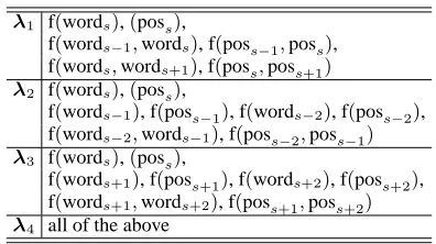
fea-λ1 f(words),(poss),
f(words−1,words), f(poss−1,poss), f(words,words+1), f(poss,poss+1) λ2 f(words),(poss),
f(words−1), f(poss−1), f(words−2), f(poss−2),
f(words−2,words−1), f(poss−2,poss−1) λ3 f(words),(poss),
f(words+1), f(poss+1), f(words+2), f(poss+2),
f(words+1,words+2), f(poss+1,poss+2) λ4 all of the above
Table 2: Features used in Chunking experiments
ture types, namely the same asλ4.
As we explained in Section 3.3, for training HySOL, the parameters of four discriminative mod-els,Λ, were trained from 4/5 of the labeled training data, and Γ were trained from remaining 1/5. For the features of the generative models, we used all of the feature types shown in Figure 1. Note that one feature type corresponds to one HMM. Thus, each HMM maintains to consist of a non-overlapping fea-ture set since each feafea-ture type only generates one symbol per state.
4.2 Syntactic Chunking Experiments
CoNLL-2000 Chunking data was obtained from the Wall Street Journal (WSJ) corpus: sections 15-18 as training data (8,936 sentences and 211,727 words), and section 20 as test data (2,012 sentences and 47,377 words), with 11 different chunk-tags, such as NP and VP plus the ‘O’ tag, which represents the region outside any target chunk.
For LOP-CRF and HySOL, we also used four base discriminative models trained by CRFs with different feature sets. Table 2 shows the feature set we used in the Chunking experiments. We used the feature set of the supplied data without any exten-sion of additional feature types.
[image:6.612.323.521.58.169.2]methods (hyper-params) Fβ=1 (gain) Sent (gain)
CRF (δ2=100.0) 84.70 - 78.30
-(4/5 labeled data,δ2=100.0) 83.74 (-0.96) 77.06 (-1.24)
[image:7.612.68.298.61.142.2]LOP-CRF (ξ0=0.1) 84.90 (+0.20) 79.02 (+0.72) HySOL (ξ0=0.1,η0=0.0001) 87.20 (+2.50) 81.19 (+2.89) (w/o prior) 86.86 (+2.16) 80.75 (+2.45) w/opGj ∀j (ξ0=1.0) 84.56 (-0.14) 78.23 (-0.07)
Table 3: NER performance (CoNLL-2003)
methods (hyper-params) Fβ=1 (gain) Sent (gain)
CRF (δ2
=10.0) 93.87 - 59.84 -(4/5 labeled data,δ2
=10.0) 93.70 (-0.17) 58.85 (-0.99) LOP-CRF (ξ0=0.1) 93.91 (+0.04) 60.34 (+0.50) HySOL (ξ0=1.0,η0=0.0001) 94.30 (+0.43) 61.73 (+1.89) (w/o prior) 94.17 (+0.30) 61.23 (+1.39) w/opG
j ∀j (ξ0=1.0) 93.84 (-0.03) 59.74 (-0.10)
Table 4: Chunking performance (CoNLL-2000)
5 Results and Discussion
We evaluated the performance in terms of the Fβ=1
score, which is the evaluation measure used in CoNLL-2000 and 2003, and sentence accuracy, since all the methods in our experiments optimize sequence loss. Tables 3 and 4 show the results of the NER and Chunking experiments, respectively. The Fβ=1and ‘Sent’ columns show the performance
evaluated using the Fβ=1 score and sentence
accu-racy, respectively. δ2,ξ andη, which are the hyper-parameters in Gaussian or Dirichlet priors, are se-lected from a certain value set by using a develop-ment set1, that is,δ2 ∈ {0.01,0.1,1,10,100,1000},
ξ−1 = ξ0 ∈ {0.01,0.1,1,10} andη −1 = η0 ∈
{0.00001,0.0001,0.001,0.01}. The second rows of CRF in Tables 3 and 4 represent the performance of base discriminative models used in HySOL with all the features, which are trained with 4/5 of the la-beled training data. The third rows of HySOL show the performance obtained without using generative models (unlabeled data). The model itself is essen-tially the same as LOP-CRFs. However the perfor-mance in the third HySOL rows was consistently lower than that of LOP-CRF since the discrimina-tive models in HySOL are trained with 4/5 labeled data.
As shown in Tables 3 and 4, HySOL
signifi-1
Chunking (CoNLL-2000) data has no common develop-ment set. Thus, our preliminary examination employed by using 4/5 labeled training data with the remaining 1/5 as development data to determine the hyper-parameter values.
[image:7.612.322.528.62.203.2]
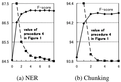
(a) NER (b) Chunking
Figure 2: Changes in the performance and the con-vergence condition value (procedure 4 in Figure 1) of HySOL.
cantly improved the performance of supervised set-ting, CRF and LOP-CRF, as regards both NER and Chunking experiments.
5.1 Impact of Incorporating Unlabeled Data The contributions provided by incorporating unla-beled data in our hybrid model can be seen by com-parison with the performance of the first and third rows in HySOL, namely a 2.64 point F-score and a 2.96 point sentence accuracy gain in the NER exper-iments and a 0.46 point F-score and a 1.99 point sen-tence accuracy gain in the Chunking experiments.
We believe there are two key ideas that enable the unlabeled data in our approach to exhibit this improvement compared with the the state-of-the-art performance provided by discriminative models in supervised settings. First, unlabeled data is only used for optimizing Equation (4) to obtain a similar effect to ’soft-clustering’, which can be calculated without information about the correct output. Sec-ond, by using a combination of generative models, we can enhance the flexibility of the feature design for unlabeled data. For example, we can handle ar-bitrary overlapping features, similar to those used in discriminative models, for unlabeled data by assign-ing one feature type for one generative model as in our experiments.
[image:7.612.68.296.176.257.2]conver-gence condition in a small number of iterations in our experiments. Moreover, the change in the per-formance remains quite stable during the iteration. However, theoretically, our optimization procedure is not guaranteed to converge in theΓandΘspace, since the optimization ofΘhas local maxima. Even if we were unable to meet the convergence condi-tion, we were easily able to obtain model parame-ters by performing a sufficient fixed number of itera-tions, and then select the parameters when Equation (4) obtained the maximum objective value.
5.3 Comparison with SS-CRF-MER
When we consider semi-supervised SOL methods, SS-CRF-MER (Jiao et al., 2006) is the most compet-itive with HySOL, since both methods are defined based on CRFs. We planned to compare the perfor-mance with that of SS-CRF-MER in our NER and Chunking experiments. Unfortunately, we failed to implement SS-CRF-MER since it requires the use of a slightly complicated algorithm, called the ‘nested’ forward-backward algorithm.
Although, we cannot compare the performance, our hybrid approach has several good characteris-tics compared with SS-CRF-MER. First, it requires a higher order algorithm, namely a ‘nested’ forward-backward algorithm, for the parameter estimation of unlabeled data whose time complexity isO(L3S2)
for each unlabeled data, whereLandSrepresent the output label size and unlabeled sample length, re-spectively. Thus, our hybrid approach is more scal-able for the size of unlabeled data, since HySOL only needs a standard forward-backward algorithm whose time complexity is O(L2S). In fact, we still have a question as to whether SS-CRF-MER is really scalable in practical time for such a large amount of unlabeled data as used in our experi-ments, which is about 680 times larger than that of (Jiao et al., 2006). Scalability for unlabeled data will become really important in the future, as it will be natural to use millions or billions of unlabeled data for further improvement. Second, SS-CRF-MER has a sensitive hyper-parameter in the objec-tive function, which controls the influence of the un-labeled data. In contrast, our objective function only has a hyper-parameter of prior distribution, which is widely used for standard MAP estimation. More-over, the experimental results shown in Tables 3 and
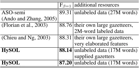
Fβ=1 additional resources
ASO-semi 89.31 unlabeled data (27M words) (Ando and Zhang, 2005)
(Florian et al., 2003) 88.76 their own large gazetteers, 2M-word labeled data (Chieu and Ng, 2003) 88.31 their own large gazetteers,
very elaborated features
HySOL 88.14 unlabeled data (17M words)
supplied gazetters
[image:8.612.311.534.60.170.2]HySOL 87.20 unlabeled data (17M words)
Table 5: Previous top systems in NER (CoNLL-2003) experiments
Fβ=1 additional resources
ASO-semi 94.39 unlabeled data (Ando and Zhang, 2005) (15M words: WSJ)
HySOL 94.30 unlabeled data
(17M words: Reuters) (Zhang et al., 2002) 94.17 full parser output (Kudo and Matsumoto, 2001) 93.91 –
Table 6: Previous top systems in Chunking (CoNLL-2000) experiments
4 indicate that HySOL is rather robust with respect to the hyper-parameter since we can obtain fairly good performance without a prior distribution.
5.4 Comparison with Previous Top Systems With respect to the performance of NER and Chunk-ing tasks, the current best performance is reported in (Ando and Zhang, 2005), which we refer to as ‘semi’, as shown in Figures 5 and 6. ASO-semi also incorporates unlabeled data solely for the additional information in the same way as our method. Unfortunately, our results could not reach their level of performance, although the size and source of the unlabeled data are not the same for cer-tain reasons. First, (Ando and Zhang, 2005) does not describe the unlabeled data used in their NER ex-periments in detail, and second, we are not licensed to use the TREC corpus including WSJ unlabeled data that they used for their Chunking experiments (training and test data for Chunking is derived from WSJ). Therefore, we simply used the supplied unla-beled data of the CoNLL-2003 shared task for both NER and Chunking. If we consider the advantage of our approach, our hybrid model incorporating gener-ative models seems rather intuitive, since it is some-times difficult to find out a design of effective auxil-iary problems for the target problem.
Fβ=1 (gain)
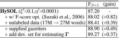
[image:9.612.80.287.61.127.2]HySOL (ξ0=0.1,η0=0.0001) 87.20 -+ w/ F-score opt. (Suzuki et al., 2006) 88.02 (-+0.82) + unlabeled data (17M→27M words) 88.41 (+0.39) + supplied gazetters 88.90 (+0.49) + add dev. set for estimatingΓ 89.27 (+0.37)
Table 7: The HySOL performance with the F-score optimization technique and some additional resources in NER (CoNLL-2003) experiments
Fβ=1 (gain)
HySOL (ξ0=0.1,η0=0.0001) 94.30 -+ w/ F-score opt. (Suzuki et al., 2006) 94.36 (-+0.06)
Table 8: The HySOL performance with the F-score optimization technique on Chunking (CoNLL-2000) experiments
from unlabeled data appear different from each other. ASO-semi uses unlabeled data for construct-ing auxiliary problems to find the ‘shared structures’ of auxiliary problems that are expected to improve the performance of the main problem. Moreover, it is possible to combine both methods, for exam-ple, by incorporating the features obtained with their method in our base discriminative models, and then construct a hybrid model using our method. There-fore, there may be a possibility of further improving the performance by this simple combination.
In NER, most of the top systems other than ASO-semi boost performance by employing exter-nal hand-crafted resources such as large gazetteers. This is why their results are superior to those ob-tained with HySOL. In fact, if we simply add the gazetteers included in CoNLL-2003 supplied data as features, HySOL achieves 88.14.
5.5 Applying F-score Optimization Technique
In addition, we can simply apply the F-score opti-mization technique for the sequence labeling tasks proposed in (Suzuki et al., 2006) to boost the HySOL performance since the base discriminative models pD(y|x) and discriminative combination, namely Equation (3), in our hybrid model basically uses the same optimization procedure as CRFs. Ta-bles 7 and 8 show the F-score gain when we apply the F-score optimization technique. As shown in the Tables, the F-score optimization technique can eas-ily improve the (F-score) performance without any additional resources or feature engineering.
In NER, we also examined HySOL with addi-tional resources to observe the performance gain. The third row represents the performance when we add approximately 10M words of unlabeled data (to-tal 27M words)2 that are derived from
1996/11/15-30 articles in Reuters corpus. Then, the fourth and fifth rows represent the performance when we add the supplied gazetters in the CoNLL-2003 data as features, and adding development data as training data of Γ. In this case, HySOL achieved a com-parable performance to that of the current best sys-tem, ASO-semi, in both NER and Chunking exper-iments even though the NER experiment is not a fair comparison since we added additional resources (gazetters and dev. set) that ASO-semi does not use in training.
6 Conclusion and Future Work
We proposed a framework for semi-supervised SOL based on a hybrid generative and discriminative ap-proach. Experimental results showed that incorpo-rating unlabeled data in a generative manner has the power to further improve on the state-of-the-art performance provided by supervised SOL methods such as CRFs, with the help of our hybrid approach, which discriminatively combines with discrimina-tive models. In future we intend to investigate more appropriate model and feature design for unlabeled data, which may further improve the performance achieved in our experiments.
Appendix
Let Vi,sD = exp(λ·fs) andVj,sG = θys−1,ysθys,xs. Equation (6) can be obtained by the following rear-rangement of Equation (2) :
R(y|x;Λ,Θ,Γ)
=
Q
ip D
i (y|x,λi)γiQjpGj(x,y,θj)γj
P
y
Q
ip D
i (y|x,λi)γi
Q
jp G
j(x,y,θj) γj
= 1
NR(x)
Y
i
£QsV D i,s Zi(x)
¤γiY
j
£ Y
s Vj,sG
¤γj
= 1
NR(x)Qi[Zi(x)]γi
Y
i
£ Y
s Vi,sD
¤γiY
j
£ Y
s Vj,sG
¤γj
= 1
NR(x)Qi[Zi(x)]γi
Y
s
Y
i
£
Vi,sD
¤γiY
j
£
Vj,sG
¤γj
.
2
References
Y. Altun, D. McAllester, and M. Belkin. 2005. Max-imum Margin Semi-Supervised Learning for Struc-tured Variables. In Proc. of NIPS*2005.
R. Ando and T. Zhang. 2005. A High-Performance Semi-Supervised Learning Method for Text Chunking. In Proc. of ACL-2005, pages 1–9.
U. Brefeld and T. Scheffer. 2006. Semi-Supervised Learning for Structured Output Variables. In Proc. of
ICML-2006.
H. L. Chieu and Hwee T. Ng. 2003. Named Entity Recognition with a Maximum Entropy Approach. In
Proc. of CoNLL-2003, pages 160–163.
A. P. Dempster, N. M. Laird, and D. B. Rubin. 1977. Maximum Likelihood from Incomplete Data via the EM Algorithm. Journal of the Royal Statistical
Soci-ety, Series B, 39:1–38.
R. Florian, A. Ittycheriah, H. Jing, and T. Zhang. 2003. Named Entity Recognition through Classifier Combi-nation. In Proc. of CoNLL-2003, pages 168–171. A. Fujino, N. Ueda, and K. Saito. 2005. A Hybrid
Gen-erative/Discriminative Approach to Semi-Supervised Classifier Design. In Proc. of AAAI-05, pages 764– 769.
Y. Grandvalet and Y. Bengio. 2004. Semi-Supervised Learning by Entropy Minimization. In Proc. of
NIPS*2004, pages 529–536.
F. Jiao, S. Wang, C.-H. Lee, R. Greiner, and D. Schuur-mans. 2006. Semi-Supervised Conditional Random Fields for Improved Sequence Segmentation and La-beling. In Proc. of COLING/ACL-2006, pages 209– 216.
T. Kudo and Y. Matsumoto. 2001. Chunking with Sup-port Vector Machines. In Proc. of NAACL 2001, pages 192–199.
J. Lafferty, A. McCallum, and F. Pereira. 2001. Condi-tional Random Fields: Probabilistic Models for Seg-menting and Labeling Sequence Data. In Proc. of
ICML-2001, pages 282–289.
W. Li and A. McCallum. 2005. Semi-Supervised Se-quence Modeling with Syntactic Topic Models. In
Proc. of AAAI-2005, pages 813–818.
D. C. Liu and J. Nocedal. 1989. On the Limited Memory BFGS Method for Large Scale Optimization. Math.
Programming, Ser. B, 45(3):503–528.
K. Nigam, A. McCallum, S. Thrun, and T. Mitchell. 2000. Text Classification from Labeled and Unlabeled Documents using EM. Machine Learning, 39:103– 134.
R. Raina, Y. Shen, A. Y. Ng, and A. McCallum. 2003. Classification with Hybrid Generative/Discriminative Models. In Proc. of NIPS*2003.
F. Sha and F. Pereira. 2003. Shallow Parsing with Condi-tional Random Fields. In Proc. of HLT/NAACL-2003, pages 213–220.
A. Smith, T. Cohn, and M. Osborne. 2005. Logarith-mic Opinion Pools for Conditional Random Fields. In
Proc. of ACL-2005, pages 10–17.
C. Sutton, M. Sindelar, and A. McCallum. 2006. Reduc-ing Weight UndertrainReduc-ing in Structured Discriminative Learning. In Proc. of HTL-NAACL 2006, pages 89–95. J. Suzuki, E. McDermott, and H. Isozoki. 2006. Training Conditional Random Fields with Multivariate Evalua-tion Measure. In Proc. of COLING/ACL-2006, pages 217–224.
E. F. Tjong Kim Sang and S. Buchholz. 2000. Introduc-tion to the CoNLL-2000 Shared Task: Chunking. In
Proc. of CoNLL-2000 and LLL-2000, pages 127–132.
E. T. Tjong Kim Sang and F. De Meulder. 2003. Intro-duction to the CoNLL-2003 Shared Task: Language-Independent Named Entity Recognition. In Proc. of
CoNLL-2003, pages 142–147.
T. Zhang, F. Damerau, and D. Johnson. 2002. Text Chunking based on a Generalization of Winnow.
Ma-chine Learning Research, 2:615–637.