Conditional Structure versus Conditional Estimation in NLP Models

Conditional Structure versus Conditional Estimation in NLP Models

Dan Klein and Christopher D. Manning

Computer Science Department Stanford University Stanford, CA 94305-9040

{klein, manning}@cs.stanford.edu

Abstract

This paper separates conditional parameter estima-tion, which consistently raises test set accuracy on statisticalNLPtasks, from conditional model struc-tures, such as the conditional Markov model used for maximum-entropy tagging, which tend to lower accuracy. Error analysis on part-of-speech tagging shows that the actual tagging errors made by the conditionally structured model derive not only from label bias, but also from other ways in which the in-dependence assumptions of the conditional model structure are unsuited to linguistic sequences. The paper presents new word-sense disambiguation and

POStagging experiments, and integrates apparently conflicting reports from other recent work.

1 Introduction

The success and widespread adoption of probabilis-tic models inNLPhas led to numerous variant

meth-ods for any given task, and it can be difficult to tell what aspects of a system have led to its relative suc-cesses or failures. As an example, maximum en-tropy taggers have achieved very good performance (Ratnaparkhi, 1998; Toutanova and Manning, 2000; Lafferty et al., 2001), but almost identical perfor-mance has also come from finely tunedHMM

mod-els (Brants, 2000; Thede and Harper, 1999). Are any performance gains due to the sequence model used, the maximum entropy approach to parameter estima-tion, or the features employed by the system?

Recent experiments have given conflicting recom-mendations. Johnson (2001) finds that a condition-ally trainedPCFGmarginally outperforms a standard jointly trained PCFG, but that a conditional shift-reduce model performs worse than a joint formu-lation. Lafferty et al. (2001) suggest on abstract grounds that conditional models will suffer from a phenomenon called label bias (Bottou, 1991) – see section 3 – but is this a significant effect for realNLP

problems?

We suggest that the results in the literature, along with the new results we present in this work, can be explained by the following generalizations:

• The ability to include better features in a well-founded fashion leads to better performance. • For fixed features, assumptions implicit in the

model structure have a large impact on errors. • Maximizing the objective being evaluated has a

re-liably positive, but often small, effect.

It is especially important to study these issues us-ing NLP data sets: NLP tasks are marked by their

complexity and sparsity, and, as we show, conclu-sions imported from the machine-learning literature do not always hold in these characteristic contexts.

In previous work, the structure of a model and the method of parameter estimation were often both changed simultaneously (for reasons of naturalness or computational ease), but in this paper we seek to tease apart the separate effects of these two factors. In section 2, we take the Naive-Bayes model, ap-plied to word-sense disambiguation (WSD), and train

it to maximize various objective functions. Our ex-periments reaffirm that discriminative objectives like conditional likelihood improve test-set accuracy. In section 3, we examine two different model structures for part-of-speech (POS) tagging. There, we ana-lyze how assumptions latent in conditional structures lower tagging accuracy and produce strange quali-tative behaviors. Finally, we discuss related recent findings by other researchers.

2 Objective Functions: Naive-Bayes

For bag-of-words WSD, we have a corpus D of la-beled examples(s,o). Each o =hoiiis a list of

nomial Naive-Bayes (NB) model (Gale et al., 1992;

McCallum and Nigam, 1998), where we assume con-ditional independence between each of the oi. This

NBmodel gives a joint distribution over the s andhoii

variables:

P(s,o)= P(s)Y

i P(oi|s)

It also implicitly makes conditional predictions:

P(s|o)=P(s,o)/X s0P(s

0_,o)

In NLP, NB models are typically used in this latter way to make conditional decisions, such as chosing the most likely word sense.1

The parameters2 = hθs;θo|sifor this model are

the sense priors P(s)and the sense-conditional word distributions P(o|s). These are typically set using (smoothed) relative frequency estimators (RFEs):

θs = P(s)=count(s)/|D|

θo|s = P(o|s)=count(s,o)/ X

o0count(s,o

0₎

These intuitive relative frequency estimators are the estimates for2which maximize the joint likelihood (JL) of D according to theNBmodel:

J L(2,D)=Y

(s,o)∈DP(s,o)

ANBmodel which has been trained to maximize JL

will be referred to asNB-JL. It is worth emphasiz-ing that, in NLPapplications, the model is typically trained jointly, then used for its P(s|o)predictions.

We can set the parameters in other ways, without changing our model. If we are doing classification, we may not care about JL. Rather, we will want to minimize whatever kinds of errors we get charged for. The JL objective is the evaluation criterion for language modeling, but a decision process’ evalua-tion is more naturally phrased in terms of P(s|o). If we want to maximize the probability assigned to the correct labeling of the corpus, the appropriate objec-tive is conditional likelihood (CL):

C L(2,D)=Y

(s,o)∈D P(s|o)

This focuses on the sense predictions, not the words, which is what we cared about in the first place.

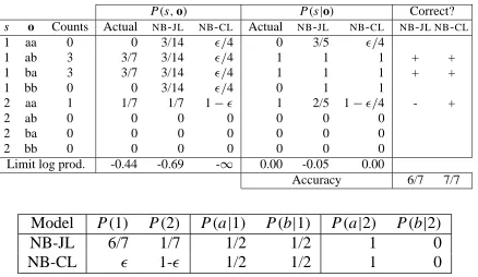
Figure 1 shows an example of the trade-offs be-tween JLand CL. Assume there are two classes (1 and 2), two words (a and b), and only 2-word con-texts. Assume the actual distribution (training and test) is 3 each of (1, ab) and (1, ba) and one (2, aa)

1_{A possible use for the joint predictions would be a}

topic-conditional unigram language model.

P(s,o) P(s|o) Correct?

s o Counts Actual NB-JL NB-CL Actual NB-JL NB-CL NB-JL NB-CL

1 aa 0 0 3/14 /4 0 3/5 /4

1 ab 3 3/7 3/14 /4 1 1 1 + +

1 ba 3 3/7 3/14 /4 1 1 1 + +

1 bb 0 0 3/14 /4 0 1 1

2 aa 1 1/7 1/7 1− 1 2/5 1−/4 - +

2 ab 0 0 0 0 0 0 0

2 ba 0 0 0 0 0 0 0

2 bb 0 0 0 0 0 0 0

Limit log prod. -0.44 -0.69 -∞ 0.00 -0.05 0.00

Accuracy 6/7 7/7

Model P(1) P(2) P(a|1) P(b|1) P(a|2) P(b|2)

NB-JL 6/7 1/7 1/2 1/2 1 0

NB-CL 1- 1/2 1/2 1 0

Figure 1: Example of joint vs. conditional estimation.

for 7 samples. Then, as shown in figure 1, the JL -maximizingNBmodel has priors of 6/7 and 1/7, like the data. The actual (joint) distribution is not in the family ofNBmodels, and so it cannot be learned per-fectly. Still, theNB-JLassigns reasonable probabili-ties to all occurring events. However, its priors cause it to incorrectly predict that aa belongs to class 1. On the other hand, maximizingCLwill push the prior for sense 1 arbitrarily close to zero. As a result, its con-ditional predictions become more accurate at the cost of its joint prediction.NB-CLjoint prediction assigns vanishing mass to events other than (2, aa), and so its joint likelihood score gets arbitrarily bad.

There are other objectives (or loss functions). In the SENSEVAL competition (Kilgarriff, 1998), we guess sense distributions, and our score is the sum of the masses assigned to the correct senses. This objective is the sum of conditional likelihoods (SCL):

SC L(2,D)=X

(s,o)∈D P(s|o)

SCL is less appropriate that CL when the model is used as a step in a probabilistic process, rather than in isolation. CL is more appropriate for filter pro-cesses, because it highly punishes assigning zero or near-zero probabilities to observed outcomes.

If we choose single senses and receive a score of either 1 or 0 on an instance, then we have 0/1-loss (Friedman, 1997). This gives the “number correct” and so we refer to the corresponding objective as

ac-curacy (Acc):

Acc(2,D)=X

(s,o)∈Dδ(s =arg maxs0P(s

0_|o))

In the following experiments, we illustrate that, for a fixed model structure, it is advantageous to max-imize objective functions which are similar to the evaluation criteria. Although in principle we can op-timize any of the objectives above, in practice some are harder to optimize than others. As stated above,

SCL, since they are continuous in 2, can be

opti-mized by gradient methods. Acc is not continuous in2and is unsuited to direct optimization (indeed, finding an optimum is NP-complete).

When optimizing an arbitrary function of 2, we have to make sure that our probabilities remain well-formed. If we want to have a well-formed jointNB in-terpretation, we must have non-negative parameters and the inequalities∀sP_oθo|s ≤ 1 andPsθs ≤ 1.

If we want to be guaranteed a non-deficient joint in-terpretation, we can require equality. However, if we relax the equality then we have a larger feasible space which may give better values of our objective.

We performed the following WSD experiments with Naive-Bayes models. We took as data the col-lection of SENSEVAL-2 English lexical sampleWSD

corpora.2 We set theNBmodel parameters in several ways. We optimizedJL (using theRFEs).3 We also optimized SCL and (the log of) CL, using a conju-gate gradient (CG) method (Press et al., 1988).4 For

CL and SCL, we optimized each objective both over

the space of all distributions and over the subspace of non-deficient models (givingCL∗andSCL∗). Acc

was not directly optimized.

UnconstrainedCLcorresponds exactly to a condi-tional maximum entropy model (Berger et al., 1996; Lafferty et al., 2001). This particular case, where there are multiple explanatory variables and a sin-gle categorical response variable, is also precisely the well-studied statistical model of (multinomial)

logistic regression (Agresti, 1990). Its optimization

problem is concave (over log parameters) and there-fore has a unique global maximum. For CL∗, SCL,

and SCL∗, we are only guaranteed local optima, but in practice we detected no maxima which were not

2_{http://www.sle.sharp.co.uk/senseval2/}

3_{Smoothing is an important factor for this task. So that the}

various estimates would be smoothed as similarly as possible, we smoothed implicitly, by adding smoothing data. We added one instance of each class occurring with the bag containing each vocabulary word once. This gave the same result as add-one smoothing on the RFEs for NB-JL, and ensured that NB

-CLwould not assign zero conditional probability to any unseen event. The smoothing data did not, however, result in smoothed estimates forSCL; any conditional probability will sum to one over the smoothing instances. For this objective, we added a penalty term proportional toPθ2, which ensured that no con-ditional sense probabilities reached 0 or 1.

4_{All optimization was done using conjugate gradient}

as-cent over log parametersλi = logθi, rather than the given parameters due to sensitivity near zero and improved quality of quadratic approximations during optimization. Linear con-straints overθ are not linear in log space, and were enforced using a quadratic Lagrange penalty method (Bertsekas, 1995).

TRAINING SET

Optimization Acc MacroAcc log J L log C L SCL

NB-JL 86.8 86.2 -22969684.7 -243184.1 4505.9

NB-CL* 98.5 96.2 -23366291.2 -973.0 5101.2

NB-CL 98.5 96.2 -23431010.0 -854.1 5115.1 NB-SCL* 94.2 93.7 -23054768.6 -226187.8 4884.4

NB-SCL 97.3 95.5 -23146735.3 -220145.0 5055.8

TEST SET

Optimization Acc MacroAcc log J L log C L SCL

NB-JL 73.6 55.0 -1816757.1 -55251.5 3695.4

NB-CL* 72.3 53.4 -1954977.1 -19854.1 3566.3

NB-CL 76.2 56.5 -1964498.5 -20498.7 3798.8

NB-SCL* 74.8 57.2 -1841305.0 -43027.8 3754.1

NB-SCL 77.5 59.7 -1872533.0 -33249.7 3890.8

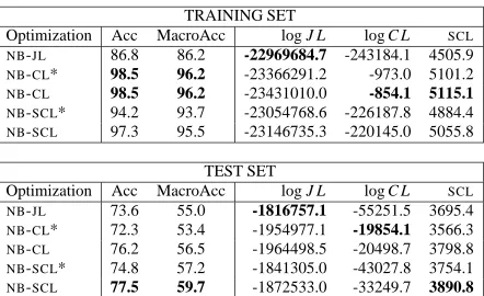
Figure 2: Scores for theNBmodel trained according to vari-ous objectives. Scores are usually higher on both training and test sets for the objective maximized, and discriminative criteria lead to better test-set accuracy. The best scores are in bold.

global over the feasible region.

Figure 2 shows, for each objective maximized, the values of all objectives on both the training and test set. Optimizing for a given objective generally gave the best score for that objective for both the training set and the test set. The exception isNB-SCLandNB -SCL* which have lower SCL score thanNB-CL and

NB-CL*. This is due to the penalty used for smooth-ing the summed models (see fn. 3).

Accuracy is higher when optimizing the discrim-inative objectives,CL and SCL, than when

optimiz-ing JL (including for macro-averaging, where each

word’s contribution to average accuracy is made equal). That these estimates beat NB-JL on

accu-racy is unsurprising, since Acc is a discretization of conditional predictions, not joint ones. This sup-ports the claim that maximizing conditional likeli-hood, or other discriminative objectives, improves test set accuracy for realistic NLP tasks. NB-SCL, though harder to maximize in general, gives better test-set accuracy than NB-CL.5 NB-CL* is some-where between JL and CL for all objectives on the training data. Its behavior shows that the change from a standardNBapproach (NB-JL) to a maximum entropy classifier (NB-CL) can be broken into two as-pects: a change in objective and an abandonment of a non-deficiency constraint.6 Note that theJLscore forNB-CL*, is not very much lower than forNB-JL, despite a large change inCL.

It would be too strong to state that maximizingCL

5_{This difference seems to be partially due to the different}

smoothing methods used: Chen and Rosenfeld (1999) show that quadratic penalties are very effective in practice, while the smoothing-data method is quite crude.

6_{If one is only interested in the model’s conditional}

-50 0 50

0 50 100 150 200 250

!

"

#$&%')(*($&%+-,.)$

/

$&(%*-0&1214325+4126

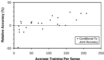
Figure 3: ConditionalNBhas higher accuracy than jointNBfor

WSD on most SENSEVAL-2 word sets. The relative improve-ment gained by switching to conditional estimation is positively correlated to training set size.

(in particular) and discriminative objectives (in gen-eral) is always better than maximizingJLfor improv-ing test-set accuracy. Even on the present task, CL

strictly beatJLin accuracy for only 15 of 24 words. Figure 3 shows a plot of the relative accuracy forCL:

(AccCL−AccJL)/AccJL. The x-axis is the average

number of training instances per sense, weighted by the frequency of that sense in the test data. There is a clear trend that larger training sets saw a larger benefit from usingNB-CL. The scatter in this trend is partially due to the wide range in data set condi-tions. The data sets exhibit an unusual amount of drift between training and test distributions. For ex-ample, the test data for amaze consists entirely of 70 instances of the less frequent of its two training senses, and represents the highest point on this graph, with NB-CL having a relative accuracy increase of

28%. This drift between the training and test cor-pora generally favors conditional estimates. On the other hand, many of these data sets are very small, individually, and 6 of the 7 sets where NB-JL wins are among the 8 smallest, 4 of them in fact being the 4 smallest. Ng and Jordan (2002) show that, between

NB-JLandNB-CL, the discriminativeNB-CLshould, in principle, have a lower asymptotic error, but the generativeNB-JL should perform better in low-data situations. They argue that unless one has a relatively large data set, one is in fact likely to be better off with the generative estimate. Their claim seems too strong here; even smaller data sets often show benefit to accuracy from CL estimation, although all would qualify as small on their scale.

Since the number of senses and skew towards common senses is so varied between SENSEVAL-2 words, we turned to larger data sets to test the ef-fective “break-even” size for WSD data, using the

hard and line data from Leacock et al. (1998).

Fig-ure 4 shows the accuracy ofNB-CLandNB-JLas the amount of training data increases. Conditional beats

0.45 0.50 0.55 0.60 0.65 0.70 0.75 0.80 0.85 0.90

0 1000 2000 3000 4000

7489:;:;< =2>?=2:@>

A

c

c

u

r

a

c

y

A)BCDEFEBCGHI4J KBECFI4J

0.79 0.80 0.81 0.82 0.83 0.84 0.85 0.86

0 1000 2000 3000 4000

LMNOPOPQ&RSTR2OUS

A

c

c

u

ra

c

y

V-WPXOTOWPNYZ4[ \WOPTZ)[

(a) (b)

Figure 4: ConditionalNBis better than JointNBforWSDgiven all but possibly the smallest training sets, and the advantage in-creases with training set size. (a) “line” (b) “hard”

joint for all but the smallest training sizes, and the im-provement is greater with larger training sets. Only for the line data does the conditional model ever drop below the joint model.

For this task, then, NB-CL is performing better than expected. This appears to be due to two ways in whichCLestimation is suited to linguistic data. First, the Ng and Jordan results do not involve smoothed data. Their data sets do not require it like linguistic data does, and smoothing largely prevents the low-data overfitting that can plague conditional models.

There is another, more interesting reason why con-ditional estimation for this model might work better for anNLPtask likeWSDthan for a general machine

learning task. One signature difficulty inNLPis that the data contains a great many rare observations. In the case ofWSD, the issue is in telling the kinds of rare events apart. Consider a wordw which occurs only once, with a sense s. In the joint model, smooth-ing ensures that w does not signal s too strongly. However, everywwhich occurs only once with s will receive the same P(w|s). Ideally, we would want to be able to tell the accidental singletons from true in-dicator words. The conditional model implicitly does this to a certain extent. Ifwoccurs with s in an ex-ample where other good indicator words are present, then those other words’ large weights will explain the occurrence of s, and withoutwhaving to have a large weight, its expected count with s in that instance will approach 1. On the other hand, if no trigger words occur in that instance, there will be no other expla-nation for s other than the presence of w and the other non-indicative words. Therefore, w’s weight, and the other words’, will grow until s is predicted sufficiently strongly.

once with each in the smoothing data). However,

transatlantic occurs in the instance thanks, anyway, the transatlantic line 2 died. , while flowers occurs

in the longer instance . . . phones with more than one

line 2, plush robes, exotic flowers, and complimen-tary wine. In the first instance, the only non-singleton

content word is died which occurs once with sense 1 and twice with sense 2. However, in the other case,

phone occurs 191 times with sense 2 and only 4 times

with sense 1. Additionally, there are more words in the second instance with which flowers can share the burden of increasing its expectation. Experimentally,

PJL(flowers|2)

PJL(flowers|1)

= PJL(transatlantic|2)

PJL(transatlantic|1)

=2

while with conditional estimation,

PCL(flowers|2)

PCL(flowers|1)

= 2.05

PCL(transatlantic|2)

PCL(transatlantic|1)

= 3.74

With joint estimation, both words signal sense 2 with equal strength. With conditional estimation, the pre-sense of words like phone cause flowers to indicate sense 2 less strongly that transatlantic. Given that the conditional estimation is implicitly differentially weighting rare events in a plausibly way, it is perhaps unsurprising that a task likeWSDwould see the ben-efits on smaller corpus sizes than would be expected on standard machine-learning data sets.7

These trends are reliable, but sometimes small. In practice, one must decide if, for example, a 5% error reduction is worth the added work: CGoptimization, especially with constraints, is considerably harder to implement than simpleRFEestimates forJL. It is also considerably slower: the total training time for the entire SENSEVAL-2 corpus was less than 3 seconds forNB-JL, but two hours forNB-CL.

3 Model Structure: HMMs and CMMs

We now consider sequence data, withPOStagging as a concreteNLPexample. In the previous section, we had a single model, but several ways of estimating parameters. In this section, we have two different model structures.

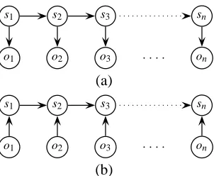
First is the classic hidden Markov model (HMM), shown in figure 6a. For an instance (s,o), where

7_{Interestingly, the common approach of discarding}

low-count events (for both training speed and overfitting reasons) when estimating the conditional models used in maxent taggers robs the system of the opportunity to exploit this effect of con-ditional estimation.

Model

Objective HMM MEMM MEMM†

JL 91.23 89.22 90.44

CL∗ 91.41 89.22 90.44

CL 91.44 89.22 90.44

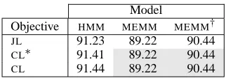
Figure 5: Tagging accuracy: For a fixed model, conditional estimation is slightly advantageous. For a fixed objective, the

MEMMis inferior, though it can be improved by unobserving unambiguous words.

o = hoiiis a word sequence and s = hsii is a tag

sequence, we write the following (joint) model:

P(s,o)=P(s)P(o|s)=Y

i P(si|si−1)P(oi|si)

where we use a start state s0to simplify notation.

The parameters of this model are the transition and emission probabilities. Again, we can set these pa-rameters to maximizeJL, as is typical, or we can set them to maximize other objectives, without chang-ing the model structure. If we maximizeCL, we get (possibly deficient)HMMs which are instances of the conditional random fields of Lafferty et al. (2001).8

Figure 5 shows the tagging accuracy of an HMM

trained to maximize each objective.JLis the standard

HMM. CL duplicates the simple CRFs in (Lafferty et al., 2001). CL∗ is again an intermediate, where we optimized conditional likelihood but required the

HMMto be non-deficient. This separates out the ben-efit of the conditional objective from the benben-efit from the possibility of deficiency (which relates to label bias, see below). In accordance with our observa-tions in the last section, and consistent with the re-sults of (Lafferty et al., 2001), the CL accuracy is slightly higher thanJLfor this fixed model.

Another model often used for sequence data is the upward Conditional Markov Model (CMM), shown

as a graphical model in figure 6b. This is the model used in maximum entropy tagging. The graphical model shown gives a joint distribution over (s,o), just like an HMM. It is a conditionally structured model, in the sense that that distribution can be writ-ten as P(s,o) = P(s|o)P(o). Since tagging only uses P(s|o), we can discard what the model says about P(o). The model as drawn assumes that each observation is independent, but we could add any ar-rows we please among the oi without changing the

conditional predictions. Therefore, it is common to think about this model as if the joint interpretation were absent, and not to model the observations at all. For models which are conditional in the sense of

8_{The general class of}

o1 o2 o3 . . . . on

s1 s2 s3 sn

(a)

o1 o2 o3 . . . . on

s1 s2 s3 sn

(b)

Figure 6: Graphical models: (a) the downwardHMM, and (b) the upward conditional Markov model (CMM).

the factorization above, theJL and CL estimates for

P(s|o)will always be the same. It is therefore tempt-ing to believe that since one can find closed-formCL

estimates (the RFEs) for these models, one can gain the benefit of conditional estimation. We will show that this is not true, at least not here.

Adopting theCMM has effects in and of itself, re-gardless of whether a maximum entropy approach is used to populate the P(s|s−1,o)estimates. The ML

estimate for this model is the RFE for P(s|s−1,o).

For tagging, sparsity makes this impossible to reli-ably estimate directly, but even if we could do so, we would have a graphical model with several defects. Every graphical model embodies conditional inde-pendence assumptions. The NBmodel assumes that

observations are independent given the class. The

HMM assumes the Markov property that future

ob-servations are independent from past ones given the intermediate state. Both assumptions are obviously false in the data, but the models do well enough for the tasks we ask of them. However, the assumptions in this upward model are worse, both qualitatively and quantitatively. It is a conditional model, in that the model can be factored as P(o)P(s|o). As a re-sult, it makes no useful statement about the distribu-tion of the data, making it useless, for example, for generation or language modeling. But more subtly note that states are independent of future observa-tions. As a result, future cues are unable to influ-ence past decisions in certain cases. For example, imagine tagging an entire sentence where the first word is an unknown word. With this model struc-ture, if we ask about the possible tags for the first word, we will get back the marginal distribution over (sentence-initial) unknown words’ tags, regardless of the following words.

We constructed two taggers. One was an HMM, as in figure 6a. It was trained for JL, CL∗, and

CL. The second was a CMM, as in figure 6b. We

used a maximum entropy model over the (word, tag) and (previous-tag, tag) features to approximate the

P(s|s−1,o) conditional probabilities. This CMM is

referred to as anMEMM. A 9-1 split of the Penn

tree-bank was used as the data corpus. To smooth these models as equally as possible and to give as unified a treatment of unseen words as possible, we mapped all words which occurred only once in training to an unknown token. New words in the test data were also mapped to this token.9

Using these taggers, we examined what kinds of errors actually occurred. One kind of error tendency in CMMs which has been hypothesized in the liter-ature is called label bias (Bottou, 1991; Lafferty et al., 2001). Label bias is a type of explaining-away phenomenon (Pearl, 1988) which can be attributed to the local conditional modeling of each state. The idea is that states whose following-state distributions have low entropy will be preferred. Whatever mass arrives at a state must be pushed to successor states; it cannot be dumped on alternate observations as in anHMM. In theory, this means that the model can get into a dysfunctional behavior where a trajectory has no relation to the observations but will still stumble onward with high conditional probability. The sense in which this is an explaining-away phenomenon is that the previous state explains the current state so well that the observation at the current state is effec-tively ignored. What we found in the case ofPOS

tag-ging was the opposite. The state-state distributions are on average nowhere near as sharply distributed as the state-observation distributions. This gives rise to the reverse explaining-away effect. The observa-tions explain the states above them so well that the previous states are effectively ignored. We call this

observation bias.

As an example, consider what happens when a word has only a single tag. The conditional distri-bution for the tag above that word will always as-sign conditional probability one to that single tag, re-gardless of the previous tag. Figure 7 shows the sen-tence All the indexes dove ., in which All should be tagged as a predeterminer (PDT).10Most occurrences of All, however, are as a determiner (DT, 106/135 vs 26/135), and it is much more common for a sentence to begin with a determiner than a predeterminer. The

9_{Doing so lowered our accuracy by approximately 2% for}

all models, but gave better-controlled experiments.

10_{The treebank predeterminer tag is meant for when words}

HMM MEMM MEMM†

Correct States PDT DT NNS VBD . -0.0 -1.3 -0.0

Incorrect States DT DT NNS VBD . -5.4 -0.3 -5.7 Observations All the indexes dove .

Figure 7: TheMEMMexhibits observation bias: knowing that the is aDTmakes the quality of theDT-DTtransition irrelevant, and All receives its most common tag (DT).

other words occur with only one tag in the tree-bank.11 The HMM tags this sentence correctly, cause two determiners in a row is rarer than All be-ing a predeterminer (and a predeterminer beginnbe-ing a sentence). However, theMEMMshows exactly the effect described above, choosing the most common tag (DT) for All, since the choice of tag for All does not effect the conditional tagging distribution for the. The MEMMparameters do assign a lower weight to

theDT DTfeature than to thePDT DTfeature, but the

the ensures aDTtag, regardless.

Exploiting the joint interpretation of the CMM,

what we can do is to unobserve word nodes, leaving the graphical model as it is, but changing the obser-vation status of a given node to “not observed”. For example, we can retain our knowledge that the state above the is DT, but “forget” that we know that the

word at that position is the. If we do inference in this example with the unobserved, taking a weighted sum over all values of that node, then the conditional dis-tribution over tag sequences changes as shown under

MEMM†: the correct tagging has once again become most probable. Unobserving the word itself is not a

priori a good idea. It could easily put too much

pres-sure on the last state to explain the fixed state. This effect is even visible in this small example: the like-lihood of the more typical PDT-DT tag sequence is even higher forMEMM†than theHMM.

These issues are quite important for NLP, since

state-of-the-art statistical taggers are all based on one of these two models. In order to check which, if ei-ther, of label or observation bias is actually contribut-ing to taggcontribut-ing error, we performed the followcontribut-ing ex-periments with our simpleHMMandMEMMtaggers. First, we measured, on the training data, the entropy of the next-state distribution P(s|s−1)for each state

s. For both theHMMandMEMM, we then measured

the relative overproposal rate for each state: the num-ber of errors where that state was incorrectly pre-dicted in the test set, divided by the overall frequency of that state in the correct answers. The label bias hy-pothesis makes a concrete prediction: lower entropy

11_{For the sake of clarity, this example has been slightly}

doc-tored by the removal of several non-DToccurrences of the in the treebank – all incorrect.

-1 -0.8 -0.6 -0.4 -0.2 0 0.2 0.4 0.6 0.8 1

0 1 2 3 4

HMM MEMM

Figure 8: State transition entropy (x-axis) does not appear to be positively correlated with the relative over-proposal frequency (y-axis) of the tags for theMEMMmodel, though it is slightly so with theHMMmodel.

states should have higher relative overproposal val-ues, especially for the MEMM. Figure 8 shows that the trends, if any, are not clear. There does appear to be a slight tendency to have higher error on the low-entropy tags for theHMM, but if there is any

su-perficial trend for theMEMM, it is the reverse. On the other hand, if systematically unobserving unambiguous observations in theMEMMled to an in-crease in accuracy, then we would have evidence of observation bias. Figure 5 shows that this is exactly the case. The error rate of the MEMM drops when

we unobserve these single-tag words (from 10.8% to 9.5%), and the error rate in positions before such words drops even more sharply (17.1% to 15.0%). The drop in overall error in fact cuts the gap between theHMMand theMEMMby about half.

The claim here is not that label bias is impossi-ble forMEMMs, nor that state-of-the-art maxent

4 Related Results

Johnson (2001) describes two parsing experiments. First, he examines a PCFG over the ATIS treebank, trained both usingRFEs to maximizeJL, and using a

CG method to maximize what we have been calling

CL∗. He does not give results for the unconstrained

CL, but even in the constrained case, the effects from section 2 occur. CL and parsing accuracy are both higher using the CL∗ estimates. He also describes a conditional shift-reduce parsing model, but notes that it underperforms the simpler joint formulation. We take these two results not as contradictory, but as confirmation that conditional estimation, though of-ten slow, generally improves accuracy, while condi-tional model structures must be used with caution. The conditional shift-reduce parsing model he de-scribes can be expected to exhibit the same type of competing-variable explaining-away issues that oc-cur inMEMMtagging. As an extreme example, if all

words have been shifted, the rest of the parser actions will be reductions with probability one.

Goodman (1996) describes algorithms for parse selection where the criterion being maximized in parse selection is the bracket-based accuracy mea-sure that parses are scored by. He shows a test-set accuracy benefit from optimizing accuracy directly.

Finally, model structure and parameter estimation are not the entirety of factors which determine the be-havior of a model. Model features are crucial, and the ability to incorporate richer features in a relatively sensible way also leads to improved models. This is the main basis of the real world benefit which has been derived from maxent models.

5 Conclusions

We have argued that optimizing an objective that is as close to the task “accuracy” as possible is advanta-geous inNLPdomains, even in data-poor cases where machine-learning results suggest discriminative ap-proaches may not be reliable. We have also argued that the model structure is a far more important issue. For simplePOStagging, the observation bias effect of the model’s independence assumptions is more evi-dent than label bias as a source of error, but both are examples of explaining-away effects which can arise in conditionally structured models. Our results, com-bined with others in the literature, suggest that con-ditional model structure is, in and of itself, undesir-able, unless that structure enables methods of incor-porating better features, explaining why

maximum-entropy taggers and parsers have had such success despite the inferior performance of their basic skele-tal models.

References

Alan Agresti. 1990. Categorical Data Analysis. John Wiley & Sons, New York.

Adam L. Berger, Stephen A. Della Pietra, and Vincent J. Della Pietra. 1996. A maximum entropy approach to natural lan-guage processing. Computational Linguistics, 22:39–71. D. P. Bertsekas. 1995. Nonlinear Programming. Athena

Scien-tific, Belmont, MA.

L´eon Bottou. 1991. Une approche theorique de l’apprentissage connexioniste; applications a la reconnaissance de la pa-role. Ph.D. thesis, Universit´e de Paris XI.

Thorsten Brants. 2000. TnT – a statistical part-of-speech tagger. In ANLP 6, pages 224–231.

S. Chen and R. Rosenfeld. 1999. A gaussian prior for smooth-ing maximum entropy models. Technical Report CMU CS-99-108, Carnegie Mellon University.

Jerome H. Friedman. 1997. On bias, variance, 0/1–loss, and the curse-of-dimensionality. Data Mining and Knowledge Discovery, 1(1):55–77.

William A. Gale, Kenneth W. Church, and David Yarowsky. 1992. A method for disambiguating word senses in a large corpus. Computers and the Humanities, 26:415–439. Joshua Goodman. 1996. Parsing algorithms and metrics. In

ACL 34, pages 177–183.

Mark Johnson. 2001. Joint and conditional estimation of tag-ging and parsing models. In ACL 39, pages 314–321. A. Kilgarriff. 1998. Senseval: An exercise in evaluating word

sense disambiguation programs. In LREC, pages 581–588. John Lafferty, Fernando Pereira, and Andrew McCallum. 2001.

Conditional random fields: Probabilistic models for seg-menting and labeling sequence data. In ICML.

Claudia Leacock, Martin Chodorow, and George A. Miller. 1998. Using corpus statistics and Wordnet relations for sense identification. Computational Linguistics, 24:147–165. Andrew McCallum and Kamal Nigam. 1998. A comparison of

event models for naive bayes text classification. In Working Notes of the 1998 AAAI/ICML Workshop on Learning for Text Categorization.

Andrew Y. Ng and Michael Jordan. 2002. On discriminative vs. generative classifiers: A comparison of logistic regression and naive bayes. In NIPS 14.

Judea Pearl. 1988. Probabilistic Reasoning in Intelligent Sys-tems: Networks of Plausible Inference. Morgan Kaufmann, San Mateo, CA.

W. H. Press, B. P. Flannery, S. A. Teukolsky, and W. T. Vetter-ling. 1988. Numerical Recipes in C. Cambridge University Press, Cambridge.

Adwait Ratnaparkhi. 1998. Maximum Entropy Models for Nat-ural Language Ambiguity Resolution. Ph.D. thesis, Univer-sity of Pennsylvania.

Scott M. Thede and Mary P. Harper. 1999. Second-order hidden Markov model for part-of-speech tagging. In ACL 37, pages 175–182.