Wavelet Based Nonstationary Wind Speed Model in Dongting Lake Cable Stayed Bridge

(1)

doi:10.4236/eng.2010.211113 Published Online November 2010 (http://www.scirp.org/journal/eng).

Wavelet-Based Nonstationary Wind Speed Model in

Dongting Lake Cable-Stayed Bridge

Xuhui He1*, Jun Fang1, Andrew Scanlon2, Zhengqing Chen3

1

School of Civil Engineering, Central South University, Changsha, China

2

Department of Civil and Environmental Engineering, The Pennsylvania State University, State College, USA

3

College of Civil Engineering, Hunan University, Changsha, China E-mail: [email protected]

Received August 28, 2010; revised October 26, 2010; accepted October 28, 2010

Abstract

The wind-rain induced vibration phenomena in the Dongting Lake Bridge (DLB) can be observed every year, and the field measurements of wind speed data of the bridge are usually nonstationary. Nonstationary wind speed can be decomposed into a deterministic time-varying mean wind speed and a zero-mean stationary fluctuating wind speed component. By using wavelet transform (WT), the time-varying mean wind speed is extracted and a nonstationary wind speed model is proposed in this paper. The wind characteristics of turbu-lence intensity, integral scale and probability distribution of the bridge are calculated from the typical wind samples recorded by the two anemometers installed on the DLB using the proposed nonstationary wind speed model based on WT. The calculated results are compared with those calculated by the empirical mode decomposition (EMD) and traditional approaches. The compared results indicate that the wavelet-based non-stationary wind speed model is more reasonable and appropriate than the EMD-based nonnon-stationary and tra-ditional stationary models for characterizing wind speed in analysis of wind-rain-induced vibration of cables.

Keywords: Time-Varying Mean Wind Speed, Nonstationary Wind Speed Model, Cable-Stayed Bridge, Wavelet Transform (WT), Wind Characteristic, Wind-Rain-Induced Vibration

1. Introduction

Under the simultaneous occurrence of moderate wind and rain, cables in cable-stayed bridges are prone to excessive and unanticipated vibration due to large flexibility, rela-tively small mass and low inherent damping have been reported in a number of cable-stayed bridges worldwide [1-3]. This vibration can cause reduced cable and connec-tion life due to fatigue or rapid deterioraconnec-tion of the corro-sion protection system and may result in the loss of public confidence in the bridge [4]. Excessive studies have been thus carried out to explore the mechanism and explain the complex phenomenon of wind-rain-induced excessive vi-bration of stay cables.

The main research methods on wind-rain-induced cable vibration include theoretical analyses [5], wind tunnel si-mulation tests [6] and field observation [1,7,8]. Some main features for wind-rain-induced vibration have been cap-tured. However, almost all previous researches were based on the assumption of considering wind as a stationary ran-dom process. In fact, the wind speed cannot keep a

statio-nary level for a long time [7] and errors may be resulted if the stationary-assumed approach is still adopted.

(2)

rea-sonable and appropriate than traditional and EMD-based approaches for characterizing wind speed in analysis of wind-rain-induced vibration of cables.

2. Wind Speed Models

2.1. Stationary Wind Speed Model

The actual wind field near the ground should include three orthogonal components such as a vertical wind speed component W t( ) , a longitudinal wind speed component U t( ), and a lateral wind speed component

( )

V t , and the descriptions of their relative characteristics. In the traditional stationary wind speed model, the boundary layer longitudinal wind speed component

( )

U t at a given height is assumed as an ergodic random process consisting of a constant mean wind speed com-ponent U, and a longitudinal fluctuating wind speed component u t( ), i.e.

( ) ( )

U t = +U u t (1)

The mean wind speed component U produces static effects on structures and the fluctuating wind speed component u t( ) produces dynamic effects. The mean wind speed denotes an average over a time interval T, which is commonly taken as 3 s, 10 min or 1 h with re-spect to wind effects on structures, leading to the so-called 3 s gust, 10 min or hourly mean wind.

0 1

( )

T

U U t dt

T

=

_∫

(2)

The mean wind speed of W t( )and V t( )are assumed zero and the relevant fluctuating wind speed components

( )

v t and w t( ) are assumed zero-mean stationary ran-dom process.

2.2. Nonstationary Wind Speed Model

Some research studies [7,9] have shown that based on field measurements, wind speed cannot maintain a statio-nary level for a long time and usually has obvious nonsta-tionary characteristics. The characteristics of nonstatio-nary random process represent that the information of time-domain, frequency-domain etc. are related with time and are not ergodic. The nonstationary wind speed can be modeled as the sum of a deterministic time-varying mean wind speed plus a zero-mean stationary random process for fluctuating wind speed [10].

*

( ) ( ) ( )

U t =U t +u t (3)

where U t( ) is a deterministic time-varying mean wind speed reflecting the temporal trend of wind speed; and

* ( )

u t is a fluctuating wind speed of a zero-mean statio-nary process. The above nonstatiostatio-nary model can be ex-panded to lateral and vertical wind speed. In fact, if wind

speed U t( ) is a strictly stationary random process, the time-varying mean wind speed U t( )will be the constant mean wind speed component U defined in Equation (1). The stationary wind speed model Equation (1) thus can be looked at as an especial case of the nonstationary model Equation (3).

3. Time-Varying Mean Wind Speed

Extraction Based on WT

3.1. Wavelet Transform

Traditional Fourier transform (FT) decomposes a signal into frequency components and determines the strength of each component. This decomposition is represented by a power spectrum of a signal. However, such an anal-ysis does not indicate if a particular frequency compo-nent of significant (local) variations occurred, and is not suitable for nonstationary signals. A short-time Fourier transform (STFT) moves a fixed-duration window over a signal and extracts the frequency content in that interval. The STFT overcomes limitations of FT and has been successfully applied in analysis of globally nonstationary signals. However, a fixed size of a filter window was found to be a limiting factor due to the resulting fixed frequency resolution.

The wavelet transform (WT) overcomes the limita-tions of FT and STFT. It can be thought of as a genera-lized STFT, with a frequency-dependent window size [11]. A wavelet family ψa b, is the set of elementary functions generated by dilations and translations of a unique admissible mother wavelet

ψ

(t):

,

1 ( )

a b

t b t

a a

ψ = ψ_ − _

  (4)

where a b, ∈R, a≠0, are the scale and translation parameters, respectively, and t is the time. At b the wavelet function is centered, and as a increases, the wavelet becomes narrower. The signal is then decom-posed into a series of basis functions of length consisting of dilated (stretched) and translated (shifted) versions of the mother function, i.e., wavelets of different scales and positions in time or space [12]. Therefore, the wavelet function can provide a good local frequency resolution for both low and high frequency components of a signal. The continuous wavelet transform (CWT) of signal

2

( ) ( )

x t ∈L R (the space of real square summable func-tions) is defined as the correction between the function

( )

x t with the family wavelet ψa b, for each a and b:

, 1

( , ) ( ) , a b

t b

W a b x t dt x

a a

ψ ψ ψ

∞ −∞

−

 

= _ _ =< >

 

∫

(5)

For special election of the mother wavelet function ( )t

ψ and for the discrete set of parameters, aj 2 j −

(3)

, 2

j j k

b = − k, with ,j k∈Z (the set of integers), the family

/ 2

, ( ) 2 (2 )

j j

j k t t k

ψ = ψ − j k, ∈Z (6)

constitutes an orthonormal basis of the Hilbert space 2

( )

L R consisting of finite-energy signals. The correlated decimated discrete wavelet transform (DWT) is obtained by

/ 2

, 2 ( ) (2 ) , ,

j j

j k j k

W =

∫

_−∞∞ x tψ t−k dt=<xψ > (7)

where j= −N,, 1,− N=log (₂ M). Equation (7) pro-vides a nonredundant representation of signal and its values constitute the coefficients in a wavelet series. These wavelet coefficients provide full information in simple way and direct estimation of local energies at different scales. Moreover, the information can be orga-nized in hierarchical scheme of nested subspaces called multiresolution analysis in 2

( )

L R . If the decomposition is carried out over all resolutions levels, the sampled signal can be expressed as below [13]:

1 1

, ,

( ) j k j k( ) j( )

j N k j N

x t W ψ t r t

− −

=− =−

=

∑ ∑

=

∑

(8)

where t=1, 2,,M , wavelet coefficients Wj k, can be interpreted as the local residual errors between succes-sive signal approximations at scales j and j+1, and

( )

j

r t is the residual signal at scale j.

3.2. Time-Varying Mean Wind Speed Extraction

Since the wavelet function family

{

ψj k, ( )t

}

is an

or-thonormal basis for 2 ( )

L R , the concept of energy is

linked with the usual notions derived from the Fourier theory. Then, the wavelet coefficients are given in Equa-tion (7), the number of coefficients at each resoluEqua-tion

level is 2j

j

N = M. Note that this correlation gives in-formation on the signal at scale 2 ,−j

and time 2 j k

− . The set of wavelet coefficients at level j,

{

C_j, ( )k

}

is also a stochastic process where krepresents the discrete time variable [14]. It provides a direct estimation of local energies at different scales. The energy at resolution lev-el is given by

2 2

,

j j j k

k

E = r =

∑

W (9)

For a complex nonstationary signal, the longest period component obtained by WT decomposing in maximum layers, is not always the optimal component reflecting the local information of nonstationary time-varying mean. Therefore, the key issue in using WT to extract the trend in nonstationary signals is how to make sure the most reasonable number of decomposition layers is consi-dered.

Based on the wavelet theory, the wavelet has the

cha-racter of conservation of energy when the wavelet func-tion is a series of orthogonal basis funcfunc-tions. For a dis-crete WT, the energy of each layer detail coefficient can be obtained using Equation (9). The appropriate levels for decomposing the time-varying mean wind speed were quantitatively determined by the sudden change of sim-ple scale wavelet energy. The accurate time-varying mean wind speed was then obtained by the inverse dis-crete orthogonal wavelet transforms of approximate coefficients [15].

3.3. Wavelet Selection and Comparison

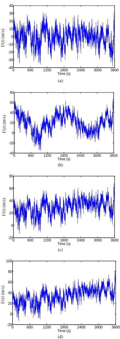
In order to verify the effectiveness and veracity of time-varying mean extraction by using WT, in this paper, a set of zero mean stationary wind speeds were simulated by adopting harmonic superposition method, as shown in

Figure 1(a). The time-varying mean value is obtained by modulating constant mean U based on different mod-ulation functions, and the nonstationary wind speed

( )

U t can be obtained by superposition of the dispersed time-varying mean value and stationary wind speed. This paper considers constant amplitude cosine function, li-near function and exponential function as constant mean modulation functions. The functions are shown in Equa-tions (10)-(12), respectively,

[

]

( ) (1 cos ), 20 / , 0, 3600

900

U t =U + π t U = m s t∈ (10)

[

]

( ) (1 / 3600), 20 / , 0, 3600

U t =U +t U= m s t∈ (11)

[

]

/3.600

( ) t , 20 / , 0, 3600

U t =Ue U= m s t∈ (12)

The time-varying mean nonstationary wind speeds by using Equations (10)-(12) are obtained and shown in

Figures 1(b)-(d), respectively.

The first step in using WT to extract time-varying mean is selecting an appropriate wavelet function family. In the wavelet tool box of MATLAT R2007, some or-thogonal wavelet families such as Daubechies wavelet, Symlets wavelet, Coiflets wavelet and Discrete Meyer wavelet can be used to extract the trend component, and some Biorthogonal and Reverse Biorthogonal wavelets can also be used for trend extraction. Since the wavelets db, and sym have compactly supported orthogonality [16], they thus adapt well to DWT. db N (N is the wavelet order number) indicates the Daubechies wavelet family with vanishing moment N, wavelet and scale functions effective supported length 2N−1; coif N

indicates the biorthogonal Coiflet wavelet family with vanishing moment N, effective supported length 2N−1 and filtering length 6N; and sym N indicates the or-thogonal Symlets wavelet family with vanishing moment

(4)

0 600 1200 1800 2400 3000 3600 -40

-30 -20 -10 0 10 20 30 40

Time (s)

U

(t

) (m/

s)

(a)

0 600 1200 1800 2400 3000 3600

-40 -20 0 20 40 60 80

Time (s)

U

(t

) (m/

s)

(b)

0 600 1200 1800 2400 3000 3600

-20 0 20 40 60 80

Time (s)

U

(t

) (m/

s)

(c)

0 600 1200 1800 2400 3000 3600

-20 0 20 40 60 80 100

Time (s)

U

(t

) (m/

s)

[image:4.595.66.276.72.661.2]

(d)

Figure 1. Original stationary wind speed and nonstationary time-varying wind speeds: (a) Original stationary wind speed; (b) Nonstationary wind speed with cosine function; (c) Nonstationary wind speed with linear function; (d) Non-stationary wind speed with exponential function.

2N. The trend extraction precision of using orthogonal wavelets of db10, coif5, sym7 and dmey are compared in this paper. By using db10 wavelet, coif5 wavelet, sym7 wavelet, dmey wavelet and the empirical mode decom-position (EMD) [17], the time-varying mean extraction of nonstatioary wind speeds shown in Figures 1(b)-(d)

are carried out, respectively. Shown in Figure 2 are the time-varying wind speeds extracted by wavelets and EMD. Table 1 lists the comparison of mean square devi-ation (MSD) between the extracted and theoretical means by using optimal wavelet functions of the 4 wavelets and EMD. From the Figure 2 and Table 1, it is seen that: 1) The MSD between the extracted and theoretical mean value obtained by EMD is much bigger than those ob-tained by all the aforementioned wavelets; 2) Among the different wavelets, the extracted precision of the un-symmetrical wavelet db10 is better than those of symme-trical wavelets coif5, ym7 and dmey, and wavelet coif5 is better than wavelet sym 7 and dmey; and 3) The ex-tracted precisions of linear function are better than cosine and exponential functions. It is found that too large or too small a wavelet order number can affect the extracted precision, and wavelet db10 has higher precision for any mean extraction. In fact, the four wavelet functions db, coif, sym7 and dmey all can be used to extract the time-varying mean wind speed. In order to gain better application effects, wavelet db10 is selected to extract the time-varying mean wind speed from the measured typical wind samples of the Dongting Lake cable-stayed bridge in this paper.

4. Description of Bridge and Field

Measurements

The Dongting Lake Bridge (DLB), as shown in Figure 3, is the first three-tower prestressed concrete cable-stayed bridge located in the influx of Dongting Lake into the Yangtze River, China. The bridge consists of two main spans of 310 m each and two side spans of 130 m each with 25.0 m clearance height above water level. The deck is 23.4 m wide with four lanes of traffic. The central tower is 125.7 m high and side towers are 99.3 m

Table 1. Comparison of MSD between extracted and theo-retical mean wind speeds.

Modulation functions

Wavelet (m/s) _EMD

(m/s)

db10 coif5 sym7 dmey

Cosine function 2.283 2.324 2.773 2.208 6.435

Linear function 0.314 0.315 0.662 0.636 3.715 Exponential

function 0.415 0.670 1.425 0.673 5.161

U

(

t

) (m

/s

)

U

(

t

) (m

/s

)

U

(

t

) (m

/s

)

U

(

t

) (m

/s

[image:4.595.310.535.634.715.2]

(5)

0 600 1200 1800 2400 3000 3600 -10

0 10 20 30 40 50 60

Time (s)

U

(t

) (m/

s)

Cosine function

Linear function

Exponential function

(a)

0 600 1200 1800 2400 3000 3600

0 10 20 30 40 50 60

Time (s)

U

(t

) (m/

s)

Cosine function Linear function Exponential function

(b)

0 600 1200 1800 2400 3000 3600

0 10 20 30 40 50 60

Time (s)

U

(t

) (m/

s)

Cosine function Linear function Exponential function

(c)

0 600 1200 1800 2400 3000 3600

-10 0 10 20 30 40 50 60

Time (s)

U

(t

) (m/

s)

Cosine function

Linear function Exponential function

(d)

Figure 2. Extracted time-varying mean wind speeds: (a) Obtained by wavelet db10; (b) Obtained by wavelet coif5; (c) Obtained by wavelet sym7; (d) Obtained by EMD.

high each. There are a total 222 cables with size ranging from 28 to 201 m in length and 99 to 159 mm in diame-ter with polyethylene (PE) pipes. Shortly afdiame-ter it opened to traffic in 2000, excessive and unanticipated wind-rain- induced cable vibrations were observed every April, July. The large-amplitude cable vibration causes concerns to the bridge administrative authority and engineers. A

Anemometer

A12 cable

South North

[image:5.595.69.271.76.588.2]

130 m 310 m 310 m 130 m

Figure 3. Elevation of Dongting Lake Bridge (DLB).

series of field observation and measurements were con-ducted, and finally MR dampers were installed on the cables (see Figure 4(a)) to mitigate cable vibration [3,7].

(a)

(b)

[image:5.595.313.539.85.141.2]

(c)

Figure 4. Dongting Lake Bridge: (a) MR dampers installed on the cables; (b) Anemometer at deck level; (c) Anemome-ter at top of south side tower.

U

(

t

) (m

/s

)

U

(

t

) (m

/s

)

U

(

t

) (m

/s

)

U

(

t

) (m

/s

[image:5.595.330.516.206.681.2]

(6)

The field tests included measurements of wind and rain characteristics, cable vibration and its mitigation by using MR dampers. Two three-axis ultrasonic ane-mometers were installed on the top of the south side tower and deck level near cable A12, respectively. Deck level one is situated at an elevation of 26 m, 4 m stretching out from the deck edge with a horizontal cantilever (see Figure 4(b)). Tower top one is situated at an elevation of 102 m, 2 m high above the tower top cantilever (see Figure 4(c)). One data acquisition and processing system in the bridge site can record the data while wind-rain-induced vibration occurs. The sample frequencies of wind speed and acceleration response are 4 Hz and 100 Hz, respectively. Continuous field measurements were conducted for 47 days from 24 March to 11 May 2003.

5. Wind Characteristics of DLB

5.1. Typical Wind Speed Samples

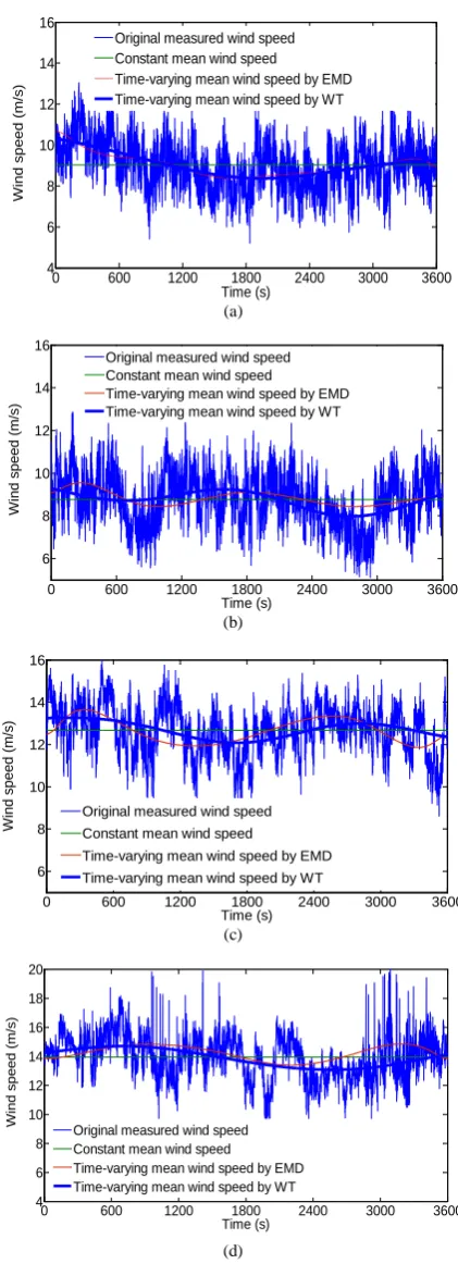
During the field testing period in 2003, significant wind-rain-induced vibrations were observed, and the corresponding wind speed and direction, rainfall and cable acceleration response data were recorded. The four typical measured wind speed data segments (1 h) from anemometers installed on the top of the south side tower and bridge deck level during wind-rain-induced vibration duration on 1 April 2003 are considered here. Shown in

Figures 5(a) and (b) are the 1h duration wind speed samples from bridge deck level anemometer between 17:10 to 18:10 and 22:20 to 23:20, 1 April 2003, respec-tively. Shown in Figures 5(c) and (d) are the 1 h dura-tion wind speed samples from the tower top anemometer between 17:10 to 18:10 and 22:20-23:20, 1 April 2003, respectively. By using the nonstationary wind speed model based on WT proposed in this paper, the time- varying mean wind speeds of the four typical wind sam-ples obtained are shown in Figures 5(a)-(d). Figures 5(a)-(d) also show the time-varying mean wind speeds obtained by EMD and the traditional constant mean wind speeds for comparison. It is seen that the mean wind speed in 1h is time-varying, and it is not appropriate to adopt the constant mean wind speed assumption. The time-varying mean wind speeds obtained by WT and EMD are a continuous function of time with a designated frequency level, which is more natural than the tradition-al time-averaged mean wind speed with the certain time interval [10]. If the traditional stationary approach is used, the errors may result in the calculated wind cha-racteristics.

0 600 1200 1800 2400 3000 3600

4 6 8 10 12 14 16

Time (s)

W

ind sp

eed (

m

/s)

Original measured wind speed Constant mean wind speed

Time-varying mean wind speed by EMD Time-varying mean wind speed by WT

(a)

0 600 1200 1800 2400 3000 3600

6 8 10 12 14 16

Time (s)

W

ind sp

eed (

m

/s)

(b)

0 600 1200 1800 2400 3000 3600

6 8 10 12 14 16

Time (s)

W

ind sp

eed (

m

/s)

Time-varying mean wind speed by EMD

Time-varying mean wind speed by WT

(c)

0 600 1200 1800 2400 3000 3600

4 6 8 10 12 14 16 18 20

Time (s)

W

ind sp

eed (

m

/s)

(d)

[image:6.595.316.527.72.654.2]

(7)

5.2. Turbulence Intensity

For stationary wind speed, the ratio of the standard devi-ation of fluctuating wind to mean wind speed is tradi-tionally defined as the turbulence intensity. The turbu-lence intensity of longitudinal fluctuating ( )u t for a given duration T is expressed by

u u I

U

σ

= (12)

with standard deviation

2 0 1

( )

T

u u t dt

T

σ =

_∫

(13)

For nonstationary wind speed, however, the mean wind speed is time varying, and turbulence intensity is also time dependent over time interval T . To be consis-tent with the turbulence intensity by the traditional me-thod, the mean value of the time varying turbulence in-tensity over the interval T

* *

( )

u u

I U t

σ

= (14)

where σ*_u means the standard deviation of fluctuating wind speed over the interval T , and u t*( )is a fluctuat-ing wind speed of a zero-mean stationary process. To have a comparison of turbulence intensities obtained by WT, EMD and traditional stationary model, the average values of longitudinal turbulence intensity of 1h duration are computed using the typical wind samples from the two anemometers installed on the bridge deck and tower top compared in Table 2. It is found that the mean values of turbulence intensities computed by nonstationary models are smaller than those obtained by the traditional stationary model. The maximum difference between the nonstationary model based on WT and traditional statio-nary model is 12.4%, and the mean difference is 9.1%. The trends of wind speed vary rapidly, as shown in Fig-ure 5, which can lead to the overestimation of turbulence intensity by the traditional stationary approach. Among the two nonstationary approaches based on WT and EMD, the results by WT are slightly smaller than those by EMD, the maximum and mean differences are 7.8% and 4.7%, respectively.

5.3. Integral Scale

Integral scales were calculated by fitting an exponen-tial curve through the autocorrelation function for each 1h sample segment. Using the typical wind samples from the two anemometers installed on the bridge deck and tower top (see Figure 5), the calculated average values of integral scale of 1h duration are com-

Table 2. Comparison of average values of longitudinal tur-bulence intensity.

Wind speed record

Nonstationary model

Stationary model Based on

WT

Based on EMD

Deck level

Sample 1 0.1296 0.1370 0.1386

Sample 2 0.1116 0.1126 0.1274

Tower top

Sample 1 0.0833 0.0870 0.0908

[image:7.595.306.541.104.200.2]

Sample 2 0.0939 0.1012 0.1036

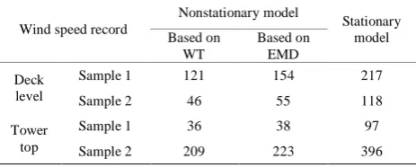
Table 3. Comparison of average values of integral scale.

Wind speed record

Nonstationary model

Stationary model Based on

WT

Based on EMD

Deck level

Sample 1 121 154 217

Sample 2 46 55 118

Tower top

Sample 1 36 38 97

Sample 2 209 223 396

puted by WT, EMD and traditional stationary approach, and compared in Table 3. Like the compared results of turbulence intensity, the average values of integral scale calculated by nonstationary models based on WT and EMD are larger than those obtained by the tradi-tional stationary model. The maximum and mean dif-ferences between the nonstationary model based on WT and traditional stationary model are 62.9%, 53.8%, respectively. The trends of wind speed vary rapidly, as shown in Figure 5, which can lead to overestimation of integral scale by the traditional stationary appr oach. Among the two nonstationary approaches based on WT and EMD, the results by WT are slightly smaller than those by EMD, the maximum and mean differences are 27.3% and 14.8%, respectively.

5.4. Probability Distribution

For stationary wind speed, the probability distribution of longitudinal fluctuating wind speed is assumed fol-low the Gaussian distribution given by

2₂ 2 1

( ) 2

u

p u e σ

πσ

−

= (15)

where σuis the standard deviation aforementioned.

[image:7.595.308.540.231.324.2]

(8)

2₂ 2 *

* 1

( )

2

u

p u e σ

πσ −

= (16)

where *

u

σ is the standard deviation of fluctuating wind speed over the interval T, and *

( )

u t is a fluc-tuating wind speed of a zero-mean stationary process. To investigate probability distributions of nonstataio-nary wind samples, four typical wind speed samples recorded at the two anemometers installed on the top of the south side tower and deck level, as shown in Fig-ure 5 are taken as examples.

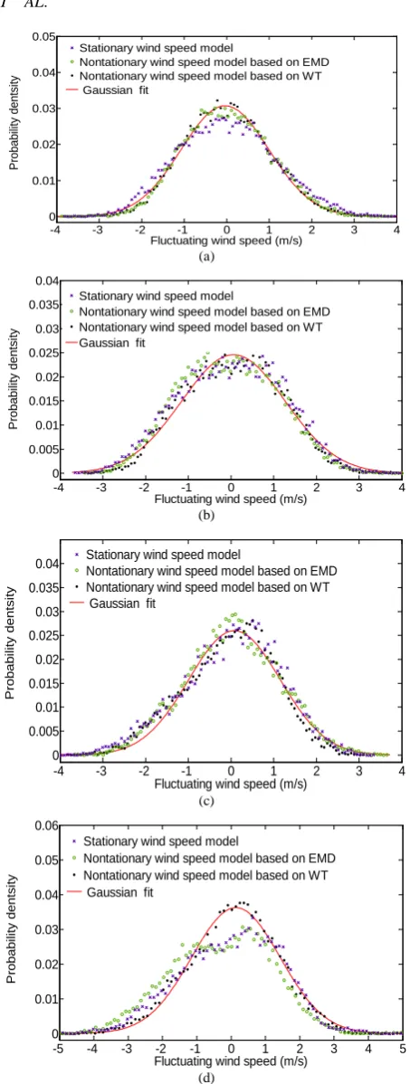
Displayed in Figure 6 are the probability distributions of two typical fluctuating wind speeds recorded from the deck level anemometer (see Figures 5(a) and (b)) and two typical fluctuating wind speeds recorded from south tower anemometer (see Figures 5(c) and (d)) together with Gaussian density functions, respectively. The prob-ability distributions based on WT are calculated from fluctuating wind speed obtained by subtracting the time-varying mean wind speed at a frequency level of 1/3600 Hz from original wind sample. The probability distributions based on EMD nonstationary and traditional stationary wind speed models are also computed and compared in Figure 6. It is seen that the probability den-sities obtained by the nonstationary model based on WT comply with the Gaussian distribution better than those calculated by nonstationary model based on EMD and traditional stationary model. Especially, as shown in

Figure 6(d), the probability distribution of the fluctuat-ing wind speed obtained based WT from tower original wind sample 2 (22:20-23:20, 1 April 2003) complies with Gaussian distribution well, but the results obtained based EMD and traditional stationary model deviate from the Gaussian distributions significantly. Thus, it may be concluded that wavelet-based stationary model is more reasonable and reliable for characterizing field measured nonstationary wind speeds.

6. Conclusions

Wind-rain-induced vibration of stay cables in cable- stayed bridge is very complicated. It is necessary to establish a reasonable wind speed model for further analysis of cable wind-rain induced vibration. A wavelet- based method for analyzing wind measurement data has been proposed in this paper. Since field measured wind samples are usually nonstationary, the proposed approach can release the limitation of stationary wind assumption of the traditional approach. The time-varying mean wind speed is more reasonable than the tradi-tional time-averaged mean wind speed for a nonstatio-nary wind speed record. Though the wavelet function selection problem of discrete orthonormal WT exists, there is a reasonable space for wavelet function

-4 -3 -2 -1 0 1 2 3 4

0 0.01 0.02 0.03 0.04 0.05

Fluctuating wind speed (m/s)

P

robabi

lit

y

dent

si

ty

Stationary wind speed model

Nontationary wind speed model based on EMD Nontationary wind speed model based on WT Gaussian fit

(a)

-4 -3 -2 -1 0 1 2 3 4

0 0.005 0.01 0.015 0.02 0.025 0.03 0.035 0.04

P

robabi

lit

y

dent

si

ty

(b)

-4 -3 -2 -1 0 1 2 3 4 0

0.005 0.01 0.015 0.02 0.025 0.03 0.035 0.04

P

robabi

li

ty

dent

si

ty

(c)

-5 -4 -3 -2 -1 0 1 2 3 4 5

0 0.01 0.02 0.03 0.04 0.05 0.06

P

robabi

li

ty

dent

si

ty

(d)

[image:8.595.309.536.61.661.2]

(9)

selection, and the influence is very limited. The analy-sis process is simple and has higher precision once an appropriate wavelet function is selected. The compari-son results indicate that wavelet db10 is the best one from the orthogonal wavelet families which can be used to extract the time-varying mean wind speed.

Based on the typical field measurement wind sam-ples recorded from the two anemometers installed on the tower top and deck level of the DLB during wind-rain-induced vibration on 1 April 2003, the time- varying mean wind speed and the wind are calculated by the nonstationary wind speed model based on WT, and the calculated results are compared with those ob-tained by the EMD nonstationary and stationary mod-els. The comparison results show that: 1) the turbu-lence intensities and integral scales of longitudinal fluctuating wind speed calculated by nonstationary wind speed models based on WT and EMD are smaller than those obtained by traditional stationary model; 2) the fluctuating wind components after wiping off the time-varying mean wind speeds from original wind records are more complied with the standard Gaussian distribution; 3) The comparison of WT and EMD indi-cates that the time-varying mean wind speed extracted by WT is more reliable and effective than EMD due to its end effect. It can be concluded that the wave-let-based method proposed in this paper is more ap-propriate than the traditional and EMD-based methods for characterizing wind speed in analysis of wind-rain- induced vibration of cables.

7. Acknowledgements

The work described in this paper was supported by the China National Science Foundation (Grant no. 50808175) to which the authors gratefully appreciate.

8. References

[1] Y. Hikami and N. Shiraishi, “Rain-Wind Induced Vibra- tions of Cables in Cable Stayed Bridges,” Journal of Wind Engineering and Industrial Aerodynamics, Vol. 29, No. 1-3, 1988, pp. 409-418.

[2] J. A. Main, N. P. Jones and H. Yamaguchi, “Evaluation of Viscous Dampers for Stay-Cable Vibration Mitigation,” Journal of Bridge Engineering, Vol. 6, No. 6, 2001, pp. 385-397.

[3] Z. Q. Chen, X. Y. Wang, J. M. Ko, Y. Q. Ni, B. F. Spencer, G. Yang and J. H. Hu, “MR Damping System for Mitigating Wind-Rain Induced Vibration on Dongting Lake Cable-Stayed Bridge,” Wind & Structures, Vol. 7, No. 5, 2004, pp. 293-304.

[4] I. Hwang, J. S. Lee and B. F. Spencer, “Isolation System for Vibration Control of Stay Cables,” Journal of Engi- neering Mechanics, Vol. 135, No. 1, 2009, pp. 61-66.

[5] D .Q. Cao, R. W. Tucker and C. Wang, “A Stochastic Approach to Cable Dynamics with Moving Rivulets,” Journal of Sound and Vibration, Vol. 268, No. 2, 2003, pp. 291-304.

[6] M. Matsumoto, N. Shirashi and H. Shirato, “Rain-Wind Induced Vibration of Cables of Cable-Stayed Bridges,” Journal of Wind Engineering and Industrial Aerodyna- mics, Vol. 43, No. 3, 1992, pp. 2011-2022.

[7] Y. Q. Ni, X. Y. Wang, Z. Q. Chen and J. M. Ko, “Field Observations of Rain-Wind-Induced Cable Vibration in Cable-Stayed Dongting Lake Bridge,” Journal of Wind Engineering and Industrial Aerodynamics, Vol. 95, No. 5, 2007, pp. 303-328.

[8] D. Zuo, N. P. Jones and J. A. Main, “Field Observation of Vortex- and Rain-Wind-Induced Stay-Cable Vibrations in a Three-Dimensional Environment,” Journal of Wind Engineering and Industrial Aerodynamics, Vol. 96, No. 6-7, 2008, pp. 1124-1133.

[9] Q. S. Li, C. K. Wong, J. Q. Fang, A. P. Jeary, and Y. W. Chow, “Field Measurements of Wind and Structural Responses of a 70-Storey Tall Building under Typhoon Conditions,” Structural Design of Tall Buildings, Vol. 9, No. 5, 2000, pp. 325-342.

[10] Y. L. Xu and J. Chen, “Characterizing Nonstationary wind Speed Using Empirical Mode Decomposition,” Journal of Structural Engineering, Vol. 130, No. 6, 2004, pp. 912-920.

[11] B. Bienkiewicz and H. J. Ham, “Wavelet Study of Approach Wind Velocity and Building Pressure,” Journal of Wind Engineering and Industrial Aerodynamics, Vol. 69-71, 1997, pp. 671-683.

[12] K. Gurley and A. Kareem, “Applications of Wavelet Trans- forms in Earthquake, Wind, and Ocean Engineering,” Engineering Structures, Vol. 21, No. 2, 1999, pp. 149- 167.

[13] O. A. Rosso, S. Blanco, J. Yordanova, V. Kolve, A. Figliola, M. Schurmann and E. Basar, “Wavelet Entropy: a New Tool for Analysis of Short Duration Brain Electrical Signals,” Journal of Neuroscience Methods, Vol. 105, No. 1, 2001, pp. 65-75.

[14] L. Zunino, D. G. Perez, M. Garavaglia and O. A. Rosso, “Wavelet Entropy of Stochastic Processes,” Physica A (Netherlands), Vol. 379, No. 2, 2007, pp. 503-512.

[15] J. H.

Varying Mean of the Non-Stationary Wind Speeds Based on Wavelet Transform (WT) and EMD,” Journal of Vibration and Shock, in Chinese, Vol. 27, No. 12, 2008, pp. 126-130.

[16] H. J. Liu, B. Q. Feng and G. C. Wu, “The Compactly Supported Cardinal Orthogonal Vector-Valued Wavelets with Dilation Factor α,” Applied Mathematics and Com- putation, Vol. 205, No. 1, 2008, pp. 309-316.