ISSN Online: 2327-5901 ISSN Print: 2327-588X
DOI: 10.4236/jpee.2019.78002 Aug. 29, 2019 27 Journal of Power and Energy Engineering
Impact of PV Distributed Generation on Loop
Distribution Network
Mohammad A. Alrumaih
1, Abdullah M. Al-Shaalan
21Saudi Electricity Company Riyadh, Riyadh, Saudi Arabia 2King Saud University Riyadh,Riyadh, Saudi Arabia
Abstract
The rapid spreading of the Photovoltaic (PV) Systems as Distributed Genera-tion (DG) in medium and low voltage networks created many effects and changes on the existing power system networks. In this work, two methods have been used and applied to determine the optimal allocation and sizing of the PV to be installed as DGs (ranging from 250 kW up to 3 MW). The first one is to determine the location according to the maximal power losses re-duction over the feeder. The second one is by using the Harmony Search Al-gorithm which is claimed to be a powerful technique for optimal allocation of PV systems. The results of the two techniques were compared and found to be nearly closed. Furthermore, investigation on the effects on the feeder in terms of voltage levels, power factor readings, and short circuit current levels has been done. All calculations and simulations are conducted by using the MATLAB Simulation Program. Some field calculations and observations have been expended in order to substantiate the research findings and validation.
Keywords
Distributed Generation (DG), Feeder, Photovoltaic System (PV), Power Factor, Ring Main Unit (RMU), Short Circuit Current, Voltage Instability
1. Introduction
The rapid growth in power demand in the Kingdom of Saudi Arabia has created many challenges to meet and satisfy that ever-growing and increasing demand. Using the fossil fuel to generate electricity will emit more harmful gases to the atmosphere and to the surrounding environment. Building huge power plants will enhance the transmission lines congestion and yield losses in the network as well. Of the proposed solutions is the Distributed Generation (DG), which is How to cite this paper: Alrumaih, M.A.
and Al-Shaalan, A.M. (2019) Impact of PV Distributed Generation on Loop Distribu-tion Network. Journal of Power and Energy Engineering, 7, 27-42.
https://doi.org/10.4236/jpee.2019.78002
Received: June 19, 2019 Accepted: August 26, 2019 Published: August 29, 2019
Copyright © 2019 by author(s) and Scientific Research Publishing Inc. This work is licensed under the Creative Commons Attribution International License (CC BY 4.0).
http://creativecommons.org/licenses/by/4.0/
DOI: 10.4236/jpee.2019.78002 28 Journal of Power and Energy Engineering
based on the idea of bringing the generation just as near as possible to the load centers. DG will not be efficient unless the generators are suitable and safe to be installed in distribution network, where the huge power generators cannot be erected and installed. DG can be defined as a small scale technology used to pro-vide source of active power, where it can be located near end-user or near to the loads in the network [1].
The size of generation which can be considered as DG is varying depending on the organization, but yet all values are convergent and not exceeding 20 MW.
Some countries have a good promising potential for wind energy like Germa-ny. Others, such as Saudi Arabia, have the availability of sunshine for most of the days. As a result of the rapid improvement in technologies for adopting renewa-ble energy facilities, Solar Photovoltaic (PV) systems account for the biggest percentage among other DG technologies. More than 90 percent of the installed distributed generation in the United States today is solar sources [2].
The presence of PV generation in distribution system has many advantages as being an environment friend, the simplicity of the system itself and the wide range of sizes which can be installed is a great advantage over the other power generation methods. From the power quality point of view, the PV systems are used in many cases to raise the bus voltage at the far end of the radial distribu-tion feeders and decreasing the losses over the feeder [3].
The main disadvantages of the DG systems are the increasing levels of short circuit current and the voltage variations and fluctuation issues. The behavior of DG itself will also have an impact on system operation and protection. The un-certainty of power flow will also increase a certain difficulty for power system protection operational setting [4].
This proposed work aims at finding the optimal allocation and sizing of the PV system to be installed in a loop distribution underground feeder [5], then, investigating and analyzing the effect of installing the PV systems on the same feeder. The PV systems are coupled to the primary bus at the distribution subs-tation which also connected to the utility system. The impact of different levels of PV penetration on voltage levels, power factor readings, and short circuit current levels will be investigated and assessed using the same distribution feed-er modeled in MATLAB simulation tool.
2. Case Study Circuit
Saudi Electricity Company (SEC) owns the whole concession of the distribution network in the Kingdom of Saudi Arabia. Furthermore, 85% of the distribution network all over the kingdom is designed and constructed similar standards [6]. Riyadh City (the Kingdom capital) constitutes nearly 15% of the overall SEC distribution network. For this reason, it has been selected to be the most appro-priate case-study application for the proposed methodology of this work.
2.1. Riyadh City Medium Voltage Network
DOI: 10.4236/jpee.2019.78002 29 Journal of Power and Energy Engineering
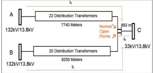
For each point on the circuit, whether it has one distribution transformer or more, a Ring Main Unit switch (RMU) is installed to maintain a high level of re-liability on the MV network. Thus, any 13.8 kV cable of the MV network can be isolated without interrupting the power supply on other equipment. Figure 1
shows a simplified single line diagram of the exciting underground loop MV network.
2.2. Network Specifications
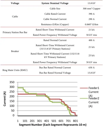
The standards used to build the MV network in Saudi Arabia were based on IEEE, IEC AEIC standards [6] [7]. Table 1 shows the specifications of the 13.8 kV network.
2.3. Case Study Circuit Specifications
The selected circuit is feeding a mixed load. 13% of the actual load in the circuit is a commercial load while 87% is a residential load.
The length of the circuit is 16,562 meters feeding 43 transformers (13.8 kV/LV). Figure 2 shows a simple topology of the circuit. Every RMU is con-necting a load to the circuit through a distribution transformer. The main cur-rents passing through the circuit are I1 and I2, while I3 is feeding only one RMU
[image:3.595.245.502.401.545.2]and planned to be as an alternative source. The current I1 and I2 are shown in
[image:3.595.238.510.579.707.2]Figure 3.
Figure 1. Single line diagram of the exciting U/G loop MV network of Riyadh City.
DOI: 10.4236/jpee.2019.78002 30 Journal of Power and Energy Engineering Table 1. 13.8 kV network specifications.
Voltage System Nominal Voltage 13.8 kV
Cable
Cable Size 300 mm2 Cupper
Cable Rated Current 390 A
Cable Normal Current 290 A
Resistance Ω/Km (Copper) 0.0607 Ω/km
Primary Station Bus Bar Rated Short-Time Withstand Current 21 kA Rated Power Frequency Withstand Voltage 50 kV rms
Breaker
Rated Normal Current 400 A
Rated Short-Time Withstand Current
(33/13.8 kV Primary Stations) 21 kA Rated Short-Time Withstand Current (132/13.8
kV Primary Stations) 25 kA
Rated Power Frequency Withstand Voltage 50 kV rms
Ring Main Units (RMU) Bus Bar Rated Normal Current 630 A Bus Bar Rated Normal Voltage 13.8 kV
Figure 3. Current reading for the two feeders over the feeder’s length.
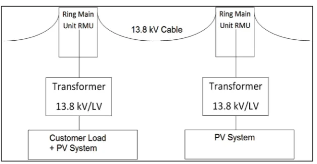
A switch (Ring Main Unit) is used to connect the PV systems to the network. This makes these PV systems more controllable by the utility company. Figure 4, shows a simplified single line diagram of the connection criteria
3. Allocation and Sizing of PV Systems
Many papers and researches have been presented on the matter of determining the allocation and sizing of the PV systems. Different methods have been intro-duced for Optimal Distributed Generation Allocation (ODGP). Three broad ap-proaches are usually used in sizing and allocation of DG units in distribution networks. These are based on analytical, numerical and heuristic methods [8].
The used numerical method in this research is to develop a MATLAB code that will calculate the power losses at each part of the distribution feeder. The distribution feeder will be divided into segments; each segment is a 10 meters
0 50 100 150 200 250 300 350
1 101 201 301 401 501 601 701 801
Cu
rr
en
t (A
)
Segment Number (Each Segment Represents 10 m)
[image:4.595.208.540.88.497.2]DOI: 10.4236/jpee.2019.78002 31 Journal of Power and Energy Engineering Figure 4. PV system connection.
long. Code’s loops will install the PV system at every segment each time, and then calculate the power losses for the whole feeder. The optimal bus to connect the PV system is the one with the least power losses for the total feeder. The method is called Maximal Power Losses Reduction. For the sake of comparison, another method will be used to determine the optimal allocation of PV system, which is Harmony Search Algorithm (HS). HS is depending on random inputs then optimizes the new results based on previous results.
3.1. Maximal Power Losses Reduction
3.1.1. Technical Work PreparationOnly Feeder 1 and Feeder 2 will be considered to install PV systems at, the spare feeder is considered to be spare. Each 10 meters is considered to be a segment, thus Feeder 1 has 774 segments and Feeder 2 has 825 segments.
The current passing through each segment consists of two elements, the cur-rent coming from primary station and the curcur-rent generated from the PV sys-tem. There are two cases:
1) The two current added together to feed the same segment as described in
Figure 5.
2) The two currents are separated; each segment is fed either from the current coming from the primary station or from the current generated from the PV system, as shown in Figure 6.
If the capacity of the PV system is more than the load, as shown in Figure 7, then, IPV, the current generated by the solar system, will be divided into two
cur-rents IPV1 and IPV2, and,
1 2
PV PV PV
I =I +I (1)
The resistance of copper cables 300 mm2 is 0.0607 Ω/Km. Thus the resistance
for each segment is 0.607 × 10⁻³ Ω/Segment. Then,
2 0.607 103
Seg Seg
PL =I × × − (2)
where PLSeg is the power lost for each segment (10 m), ISeg is the current
DOI: 10.4236/jpee.2019.78002 32 Journal of Power and Energy Engineering Figure 5. Added primary station current and solar system current.
Figure 6. Primary station current and solar system current are separated.
Figure 7. Maximal power loss reduction process flowchart.
DOI: 10.4236/jpee.2019.78002 33 Journal of Power and Energy Engineering
3 . .
Seg Seg
Connected Load IL
p f V =
× × (3)
where Connected LoadSeg is the connected load for each segment (kW), which
is provided from Saudi Electricity Company SEC data, as shown in Figure 5,
. .
p f is the Power factor, V is the voltage (V).
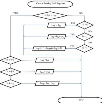
A loop is created to change the location of PV system and install it at a specific segment in each loop iteration. This loop is called PV location loop (i). A second loop initiated to calculate the power losses at each segment, which called seg-ment power losses loop (j).
The primary station current which is feeding part of the feeder is equal to:
291.82
PS PV
I = −I (4)
where IPS is the current coming from the primary station (A), IPV is the current
generated from the PV system (A), 291.82 is the actual reading of current of Feeder 1 (A), for feeder 2, the actual reading of current 228.48 A.
If i = j, means the iteration of PV system location and the iteration of segment power losses are equal. The current passing through the segment will be equal to:
Seg PS PV
I =I +I (5) If i > j, then the current passing the segment will be:
Seg PS
I =I (6)
which means that the segments before the location of installing the PV system are feeding only from the primary station source.
If i < j, then the current passing the segment will be the difference in current in previous segment, to find the current passing the next segment:
(
1)
( )
( )
(
1)
3 . . 3 . .
Seg Seg
Seg Seg
Total Load Total Load
I j I j j j
p f V p f V
+ = − − −
× × × ×
(7)
where the total load is the summation of power losses and the actual load of the segment,
Seg Seg Seg
Total load =Connected Load +PL (8)
The last part of the feeder where the current feeding the load, is only the cur-rent generated from the PV system, as shown in Figure 7. The segment K is considered to be the first segment to be fed by IPV. In other words, the point K is
the point which after it only IPV is feeding the circuit. The equations will be
dif-ferent since the current direction is difdif-ferent. There are three cases to be consi-dered:
1) K = j = i
In this case,
Seg PV
I =I (9)
DOI: 10.4236/jpee.2019.78002 34 Journal of Power and Energy Engineering
(
)
( )
( )
(
1)
3 . . .
1
3 .
Seg Seg
PV PV
Total Load Total Load
I I j j
p f V p f V
j+ j − −
× × ×
−
×
= (10)
2) K < j < i
In the case when the iteration of (j) is smaller than the iteration of (i), the current passing each segment will be calculated using the following equations,
3 . .
j Seg Seg K Seg Connected Load IL
p f V =
=
× ×
∑
(11)
The power loss is calculated after that by Equation (2), and then the total power of the segment is equal to,
j
Seg Seg K Seg Seg
Total Power =
∑
= Connected Load +PL (12)Then IPV1 is calculated using the following equation,
1
3 . .
Seg PV
Total power I
p f V × =
× (13)
And,
(
1)
( )
( )
(
1)
3 . . 3 . .
Seg Seg
Seg Seg
Total Load Total Load
I j I j j j
p f V p f V
+ = + − −
× × × ×
(14)
3) K< i < j
If the iteration of PV system location (i) is smaller than the iteration of the segment power losses (j),
2 1
PV PV PV
I =I −I (15) The PV system will be installed at a specific segment, and then the power losses will be calculated for each segment. The total power losses of the feeder are determined by adding all the power losses in all segments. After that, the lo-cation of PV system will be changed to the next segment and then the power losses of the feeder will be calculated using the same procedure.
Different sizes of the PV system will be studied, 0.25, 0.5, 0.75, 1, 1.5, 2, 2.5 and 3 MW. Figure 7 illustrates the process.
3.1.2. Feeder 1 Result
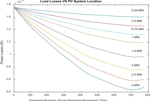
Multiple situations of connecting several sizes of PV systems have been studied. The calculation is done based on the peak load. For example, if a 1 MW PV sys-tem were installed in Feeder 1 of the circuit, the optimal location would be at segment 715 (means at 7150 m). The power loss of MV cable in Feeder 1 of the circuit would record 11.961 kW, while the total load of Feeder 1 is 6.277 MW. The losses percentage is 0.1908%. Figure 8 shows numbers of cases which were studied to determine the optimal location of the PV systems.
DOI: 10.4236/jpee.2019.78002 35 Journal of Power and Energy Engineering Figure 8. Optimal bus to connect the PV systems (Feeder 1).
PV system gets smaller, the optimal location gets further in the feeder. The slope of the line increased sharply at three locations. The first one is between segment 100 and 200, the second location is between segment 400 and 500, and the last one is at the end of the feeder. The reason is the concentration of load at these locations. As the curves reach the end of the feeder, the slope change its direc-tion to rise up, means the power loss start to increase as the installed PV system location gets further after the optimal location. Table 2 summarizes the results.
Table 2 illustrates that as the total PV systems get smaller, the optimal place would be at the end of the feeder. The power loss is decreasing as the installed PV systems getting bigger. The differences between the optimal locations for each case related to the load distribution over the feeder. Similarly, the differ-ences in power loss are related to the same reason. The result would be different based on the distribution of the load over the feeder and the length of the cable.
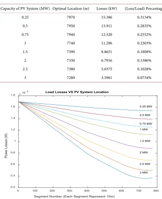
3.1.3. Feeder 2 Result
For Feeder 2 of the circuit, in all the cases, the optimal location to install a PV system of size 3 MW or less is at the end of the feeder.
As the capacity of the PV system increase the power loss of the feeder de-crease. The optimal location is changing as the capacity of the PV system changes, see Figure 9. As the installed capacity of PV system gets smaller, the optimal location gets further in the feeder. The slope of the line kept constant till it reaches segment 370, where the part before is a load free. The slope increased at two locations, between segment 370 and 450, the second location is from seg-ment 570 to nearly 700. The reason is because of the concentration of load at these locations. For the 2.5 and 3 MW systems capacity, as the curves reach the end of the feeder, the slope changes its direction to rise up, means the power loss start to increase as the installed PV system location gets further after the optimal location, just like the situation in Feeder 1. Table 3 summarizes the result.
0 100 200 300 400 500 600 700 800
Segment Number (Each Segment Represent 10m) 0.4
0.6 0.8 1 1.2 1.4 1.6 1.8
Power Losses (W)
104 Load Losses VS PV System Location
DOI: 10.4236/jpee.2019.78002 36 Journal of Power and Energy Engineering Table 2. Feeder 1 results summary.
Capacity of PV System (MW) Optimal Location (m) Losses (kW) (Loss/Load) Percentage
0.25 7330 16.050 0.2559%
0.5 7210 14.610 0.2330%
0.75 7210 13.245 0.2113%
1 7150 11.961 0.1908%
1.5 7130 9.6131 0.1534%
2 6940 7.6090 0.1215%
2.5 6920 5.8802 0.0939%
[image:10.595.211.531.268.660.2]3 6920 4.4462 0.0710%
Table 3. Feeder 2 results summary.
Capacity of PV System (MW) Optimal Location (m) Losses (kW) (Loss/Load) Percentage
0.25 7970 15.386 0.3134%
0.5 7950 13.911 0.2835%
0.75 7940 12.520 0.2552%
1 7740 11.296 0.2303%
1.5 7390 8.8651 0.1808%
2 7330 6.7916 0.1386%
2.5 7380 5.0375 0.1028%
3 7280 3.5961 0.0734%
Figure 9. Optimal bus to connect the PV systems (Feeder 2).
Table 3 illustrates that as the total PV systems get smaller, the optimal place would be at the end of the feeder. The power loss is decreasing as the installed
0 100 200 300 400 500 600 700 800
Segment Number (Each Segment Represent 10m) 0.2
0.4 0.6 0.8 1 1.2 1.4 1.6 1.8
Power Losses (W)
104 Load Losses VS PV System Location
DOI: 10.4236/jpee.2019.78002 37 Journal of Power and Energy Engineering
PV systems getting bigger. As shown in the table, all optimal locations are de-termined to be at the furthest segments, which are much predicted based on the load distribution over the feeder. The result would be different based on the dis-tribution of the load over the feeder and the length of the cable.
3.2. Harmony Search Algorithm
The HS algorithm, which is based on random inputs, is used also to find the op-timal allocation of PV system. A MATLAB code was developed to apply the harmony search algorithm. A system of 1 MW is installed in both Feeder 1 and 2. Table 4, summarizes the results,
The HS algorithm results are comparable for the two feeders. For the first feeder of the circuit, the optimal location of installing a 1 MW PV system is the same location resultant by two methods, whereas, for the second feeder, the op-timal locations were different but they are close to each other. For the power loss percentage, the results were very close to the two methods.
4. The Impact of the Connected PV Systems on Power
System Stability
The rapid expansion of electrical network requires improvement of the quality and reliability of power system. Voltage stability is a major issue which affects the end-users especially in the industrial sector. Connecting another source to the network would have its effect on stability of the power system [9]. The fault current values would also be affected by the penetration of DG [10].
After defining the optimal placement of PV systems in terms of circuit power loss, the impact of connecting the PV system is studied. This research is focusing on the impact on voltage instability, power factor and fault current calculation.
The used simulation program is MATLAB through Simulink tool. The case study circuit is modeled then tested.
4.1. Impact on Voltage Instability
[image:11.595.211.540.632.732.2]A fundamental requirement in the operation of a power system is that power flow and bus voltages are maintained within acceptable limits throughout the network despite changes in load or available transmission and generation re-sources. Furthermore, the system needs to exhibit an ability to remain in a state of operating equilibrium under normal operating conditions and to regain an
Table 4. Compression between the two methods.
Method Feeder Location (m) Optimal Losses (kW) (Loss/Load) Percentage
Maximal Power Loss Reduction
Feeder 1 7200 11.956 0.1908%
Harmony Search Algorithm 7200 11.989 0.1911%
Maximal Power Loss Reduction
Feeder 2 7740 11.296 0.2303%
DOI: 10.4236/jpee.2019.78002 38 Journal of Power and Energy Engineering
acceptable state of equilibrium after being subjected to a disturbance. The dis-turbance may be associated with an outage of a generator, transformer, line or loads [11].
Several PV systems were connected to the feeders, ranging from 0.25 MW up to 1 MW. Table 5 shows the percentage of improvement of voltage at the far end bus for each feeder.
The voltage measurements after connecting 0.25, 0.5, 0.75 and 1 MW PV sys-tem increased by a small percentage which is reasonable based on the capacit-ance nature of the underground cables and the length of the cable. The effect would be different if a larger capacity PV system was connected to the feeder, or if the characteristic of the feeders is different.
4.2. The Effect on Power Factor
Power quality is one of the main concerns of both power plant owners and Net-work System Operators [12].
In reference [13], the researcher considered a 69-bus, 8-lateral distribution feeder. He considered four different PV penetrations: 190 kW, 380 kW, 570 kW and 760 kW. Assuming that all PV systems are multiples of the standard PV “building block” of 2 kW, i.e. for a 760 kW PV penetration, 380 “building blocks” are scattered across the feeder.
A significant improvement of nearly 3% increasing happened to the power factor over the substation level. The reasons are because of the characteristic of the feeder itself, length, load distribution, etc. The second reason is the optimal distribution of small sizes PV system across the feeder [13].
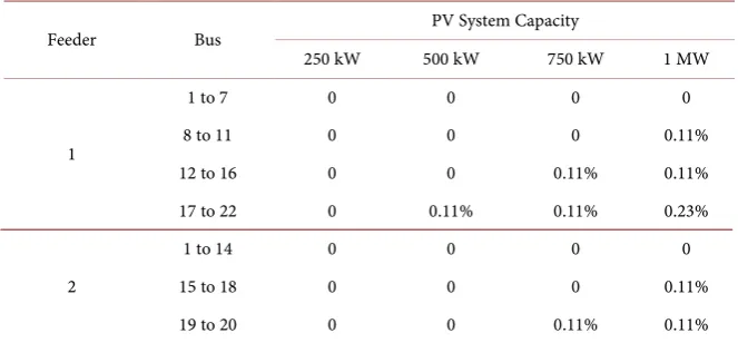
For the case study circuit of this research, the PV system is installed at one op-timal location defined in the first part of the research. The exciting power factor measured at the load end, without connecting the PV system, it was ranging from 0.86 up to 0.93. Table 6 shows the percentage of improvement of power factor value.
[image:12.595.207.540.621.738.2]Although the improvement is a very slight and it will not reflect a huge im-provement, but in the long period, it will help to reduce the losses. In Feeder 2 of the circuit, no bus had experienced an improvement of 0.0002 in p.f. reading, which is reasonable due to the concentration of load at the end of the feeder. Due to the installation PV system in one location of the circuit, the readings of power factor for both feeders did not improve significantly as in reference [13],
Table 5. Percentage of improvement after connecting the PV system.
Bus PV System Capacity
250 kW 500 kW 750 kW 1 MW
Feeder 1
22 0.66% 0.66% 0.73% 0.81%
Feeder 2
DOI: 10.4236/jpee.2019.78002 39 Journal of Power and Energy Engineering Table 6. Power factor’s percentage of improvement.
Feeder Bus PV System Capacity
250 kW 500 kW 750 kW 1 MW
1
1 to 7 0 0 0 0
8 to 11 0 0 0 0.11%
12 to 16 0 0 0.11% 0.11%
17 to 22 0 0.11% 0.11% 0.23%
2
1 to 14 0 0 0 0
15 to 18 0 0 0 0.11%
19 to 20 0 0 0.11% 0.11%
which had several small sizes of PV systems distributed over the case-study feeder.
The customers will also be benefits as they are paying only for the active pow-er. This improvement will reduce the reactive power in the circuit. The low power factor causes the utility to have to increase its generation and transmis-sion capacity in order to handle this extra demand. By raising the power factor, the consumption of reactive power will be less. This results in less active in KW, which equates to a money savings for both the utility company and the custom-ers [14].
4.3. The Impact on Protection
Introduction of DG to the traditional power systems changes the radial passive distribution network into active network. Thus, it changes the value of fault cur-rent and duration, the curcur-rent flow no longer unilaterally from the grid station bus flows into the load. The failure behavior of DG itself also will have an impact on system operation and protection [11]. In the case of a short circuit on the network, the short circuit current could theoretically be partly provided by the PV generator, which would disturb the detection of the fault by the protection devices provided on the network.
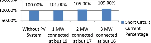
The PV system is installed at the optimal location defined by the maximum loss reduction. Since the occurrence of the three phase fault represented the highest impact on the short circuit level, it is considered in this research. Three cases were studied, 1 MW, 2 MW and 3 MW systems were connected respectively.
1) Feeder 1
For the first feeder of the circuit, the optimal location of connecting the PV system is at bus 18 for a 1 MW system at bus 16 for both 2 MW and 3 MW sys-tems. Figure 10 shows the percentage of short circuit current increasing.
DOI: 10.4236/jpee.2019.78002 40 Journal of Power and Energy Engineering
7%. While a 3 MW PV system would result in an increasing of short circuit cur-rent value by 7.5%. These results will not affect the network design specification since such an increase in the fault current is already counted. The increasing in short circuit current value was affected by the location of PV system. If the ca-pacity of the PV increases, the optimal location will be closer to the primary sta-tion; thus the short circuit current will be higher.
2) Feeder 2
For the second part of the circuit, the optimal location of connecting the PV system is at bus 19 for a 1 MW system, at bus 17 for a 2 MW, while for a 3 MW systems, the optimal location is at bus 16.
As shown in Figure 11, the short circuit current increased when PV system is erected to the feeder. When connecting a 1 MW PV system, the value of short circuit current at the connection bus increased by 1%. If the connected PV sys-tem is a 2 MW syssys-tem then, the short circuit current value will be increased by 5%. While a 3 MW PV system would result in an increasing of short circuit cur-rent value by 9%. These results will not affect the network design specification since such an increase in the fault current is already counted. The increasing in short circuit current value was affected by the location of PV system. If the ca-pacity of the PV increases, the optimal location will be closer to the primary sta-tion; thus the short circuit current will be higher.
[image:14.595.223.528.435.547.2]Generally, it is considered that PV generators connected to distribution net-works do not contribute significantly to short circuit fault current, in case such events occur on the distribution system side. This is because the short-circuit
Figure 10. The percentage of short circuit current increasing due to PV system connect-ing for Feeder 1.
Figure 11. The percentage of short circuit current increasing due to PV system connect-ing for Feeder 2.
100.00% 101.00% 107.00% 107.50%
50.00% 100.00% 150.00%
Without PV
System connected 1 MW at bus 18
2 MW connected
at bus 16
3 MW connected
at bus 16
Short Circuit Current Percentage
100.00% 101.00% 105.00% 109.00%
50.00% 100.00% 150.00%
Without PV
System connected 1 MW at bus 19
2 MW connected
at bus 17
3 MW connected
at bus 16
[image:14.595.223.529.605.693.2]DOI: 10.4236/jpee.2019.78002 41 Journal of Power and Energy Engineering
current of a PV array is 10% - 20% more than the rated maximum output rent at most, inverters are normally equipped with under voltage relays and cur-rent controlled types mainly used in PVDG have over-curcur-rent limiting in case of disturbances on the distribution system side.
From the results above of short circuit current values with and without the interconnection of PV systems, it is obvious that there is no significant impact would be introduce by interconnecting a PV systems of less than 3 MW to such feeders.
5. Conclusion
The aim of this proposed work is to identify the optimal locations of PV systems ranging from 250 kW up to 3 MW to be connected and integrated to the MV network. A typical underground 13.8 kV circuit among Riyadh City network was selected to be the case study application. The circuit consists of three feeders, two of them are main source of power and the third is a spare one. The main two feeders were implemented in the research. The used method is a numerical one which tries all the possibilities and gives the optimal location based on maximal power loss reduction. The simulation was done using a unique MATLAB code. A heuristic method which is the Harmony Search Algorithm (HAS) was used to determine the optimal location and compare the two results. Some field experi-mental observations and calculations using the HAS were also performed and documented. In both feeders the result were comparable, the optimal locations for connecting the PV system were at the end of each feeder, or specifically, at load point side. The optimal location is getting as closer as possible to the power source as the system capacity becomes larger.
Conflicts of Interest
The authors declare no conflicts of interest regarding the publication of this pa-per.
References
[1] Nasir, M., Shahrin, N., Bohari, Z., Sulaima, M. and Hassan, M. (2014) A Distribu-tion Network ReconfiguraDistribu-tion Based on PSO: Considering DGs Sizing and Alloca-tion EvaluaAlloca-tion for Voltage Profile Improvement. IEEE Student Conference on Re-search and Development, Penang, 16-17 December 2014.
https://doi.org/10.1109/SCORED.2014.7072981
[2] American Public Power Association (2013) Distributed Generation. Washington DC.
[3] Heydt, G.T. (2010) The Next Generation of Power Distribution Systems. IEEE Transactions on Smart Grid, 1, 225-235. https://doi.org/10.1109/TSG.2010.2080328
[4] Ezysolare.com (2016) Trend Analysis on Solar PV Module Prices.
http://www.ezysolare.com/blog/knowledge-center/trend-analysis-on-solar-pv-mod ule-prices
De-DOI: 10.4236/jpee.2019.78002 42 Journal of Power and Energy Engineering
finition. Electric Power Systems Research, 57, 195-204. https://doi.org/10.1016/S0378-7796(01)00101-8
[6] Saudi Electricity Company (2015) Transmission Materials Standard Specifications No. 01-TMSS-01 REV.02. Riyadh.
[7] Saudi Electricity Company (2013) SEC Distribution Materials Specifications No. 11-SDMS-03 REV.02. Riyadh.
[8] Labrini, H., Gad, A., ElShatshat, R.A. and Salama, M.M.A. (2015) Dynamic Graph Based DG allocation for Congestion Mitigation in Radial Distribution Networks.
IEEE Power & Energy Society General Meeting, Denver, 26-30 July 2015. https://doi.org/10.1109/PESGM.2015.7286611
[9] Kuang, H., Li, S. and Wu, Z. (2011) Discussion on Advantages and Disadvantages of Distributed Generation Connected to the Grid. International Conference on Elec-trical and Control Engineering, Yichang, 16-18 September 2011.
[10] Gurkiran, K. and Mohammad, V. (2006) Effects of Distributed Generation (DG) Interconnections on Protection of Distribution Feeders. Power Engineering Society General Meeting, Montreal.
[11] Chiradeja, R. and Ramakumar, R. (2004) An Approach to Quantify the Technical Benefits of Distributed Generation. IEEE Transactions on Energy Conversion, 19, 764-773.https://doi.org/10.1109/TEC.2004.827704
[12] Camacho, A., Castilla, M., Miret, J., Matas, J., Guzman, R., Sousa-Pérez, O., Martí, P. and García de Vicuña, L. (2013) Control Strategies Based on Effective Power Factor for Distributed Generation Power Plants during Unbalanced Grid Voltage. 39th Annual Conference of the IEEE, Vienna, 10-13 November 2013.
https://doi.org/10.1109/IECON.2013.6700318
[13] Begovic, M., Pregelj, A., Rohatgi, A. and Novosel, D. (2001) Impact of Renewable Distributed Generation on Power Systems. Proceedings of the Hawaii International Conference on System Sciences, Maui, 6 January 2001.
[14] Lucian, L., Dulăua, M. and Abrudean, D. (2013) Effects of Distributed Generation on Electric Power Systems. The 7th International Conference Interdisciplinarity in Engineering, Târgu Mureș, 10-11 October 2013.
Nomenclature
Loop Distribution Network can be seen as a medium voltage network topology where the circuit is connected in loop with the existing of Normal Open Point (NOP) for each circuit to avoid the load flow and keep only one source of cur-rent which can be changed operationally by switching ON and OFF the RMU switches either manually or automatically.