A Hyperbolic Eulerian Model for Dilute Two Phase Suspensions

A Hyperbolic Eulerian Model for Dilute Two-Phase

Suspensions

Sarah Hank, Richard Saurel, Olivier Le Metayer IUSTI, Aix Marseille University, Marseille Cedex, France

Bastidon de la Caou, Roquevaire, France

E-mail:{Sarah.Hank, Richard.Saurel, Olivier.Lemetayer}@polytech.univ-mrs.fr Received May 4, 2011; revised June 22, 2011; accepted July 1, 2011

Abstract

Conventional modeling of two-phase dilute suspensions is achieved with the Euler equations for the gas phase and gas dynamics pressureless equations for the dispersed phase, the two systems being coupled by various relaxation terms. The gas phase equations form a hyperbolic system but the particle phase corre-sponds to a hyperbolic degenerated one. Numerical difficulties are thus present when dealing with the dilute phase system. In the present work, we consider the addition of turbulent effects in both phases in a thermo-dynamically consistent way. It results in two strictly hyperbolic systems describing phase’s dynamics. An-other important feature is that the new model has improved physical capabilities. It is able, for example, to predict particle dispersion, while the conventional approach fails. These features are highlighted on several test problems involving particles jets dispersion and are compared against experimental data. With the help of a single parameter (a turbulent viscosity), excellent agreement is obtained for various experimental con-figurations studied by different authors

Keywords: Turbulence, Riemann Solver, Pressureless Gas Dynamics

1. Introduction

Two phase diluted flows are present in many fundamen-tal and industrial applications ranging from astrophysics, fluid mechanics, chemical engineering, combustion, nu-clear engineering and so on. The Eulerian approach is widely used to deal with such flows, considering velocity non-equilibrium effects in a two-fluid description. It considers the gas phase governed by the Euler or Navier- Stokes equations where the volume occupied by the par-ticles is neglected, and the dispersed phase (solid or liq-uid) governed by the pressureless gas dynamics equa-tions [1,2]. The coupling between those two sub-systems is achieved with relaxation terms expressing drag forces, heat and mass transfer effects. The dispersed phase sys-tem (pressureless gas dynamics equations) poses how-ever serious difficulties. It is not possible to express the equations in characteristic variables as there is no set of independent eigenvectors. Shocks are unconventional as they don’t respect the sub-characteristic criterion [3]. These theoretical difficulties induce computational ones, as for example the treatment of reflective boundary con-ditions as well as any situation involving crossing

998 S. HANK ET AL. particles turbulence is present, dispersion occurs

result-ing in jet enlargement in perfect agreement with experi-mental measurements if proper turbulent viscosity is used.

The present paper is organized as follows. The con-ventional two-fluid model with pressureless equations for the particle phase is recalled in Section 2. Then tur-bulent effects are modeled in Section 3 with the thermo-dynamic method given in [7]. The Riemann problem solution for the particles system is examined in Section 4, and those of the gas phase is considered in Section 5. Dissipative effects including relaxation ones and turbu-lent viscosity are inserted in Section 6. They result in turbulence production in both phases. Section 7 deals with some details about numerical implementation. Sev-eral test problems and comparison between the conven-tional pressureless model and the new turbulent model are considered in Section 8, first in one dimension, then in two dimensions, allowing comparisons with experi-mental data of free jet particle flows in air. Conclusions are given in Section 9.

2. Conventional Eulerian Flow Model for

Dilute Suspensions

The following flow model considers each phase as a continuous media. In the carrier phase, molecular colli-sions are so intense that pressure appears as an external force to a given gas control volume. In the dispersed phase, the collisions are less intense and are here consid-ered as negligible. This assumption is reasonable as the particle volume concentration is weak [8], say

2

10 p

 _ 

where p represents the dispersed phase volume

frac-tion. In addition, neglecting the volume occupied by the particles for the gas flow results in the following system [1,2]. The evolution equations for carrier phase are the following ones,

( ) 0

( ) (

( ) ( )

p)

p p

u t

u _{u u PI u u}

t E

Eu Pu u u u

t

 _

 _{ }

 _{ }



 _{  }

  



 _{      }

 _ 



 _{      }

  

 

   

    

(1)

and for the dispersed phase,

( ) 0

( ) (

( ) ( )

p

p p

p p

p p p p

p p

p

 represents the particles apparent density,  p

*

p

  , where _* _{represents the condensed phase real} density (considered here as incompressible). The total energies are defined by:

2

2 u

E e 



and

2

2 p

p p

u

E e 



.

In the carrier phase system, there is a coupling be-tween the internal energy ( ), the density (e  ) and the pressure (P) with the help of a convex equation of state (EOS):

( , )

P P  e .

In the dispersed phase, such coupling is absent. The particles are incompressible and collisional effects are neglected. The only interaction force considered here is the drag force, modeled by the velocity relaxation pa-rameter λ> 0. The power of the drag force is assumed to be transferred with the particles velocity, resulting in entropy production in the gas, and isentropic evolutions in the particles:

2 ( )

( ) 0

p

p p

p p p

s

us u u

t T

s

u s t

0

 _ 





 _{    }

 

  



  



It can be shown easily that the gas dynamic system is strictly hyperbolic with waves speed u, u + c and u – c. The sound speed c is defined by,

2 _/

c P 

where γ represents the specific heats ratio.

The particles phase system is hyperbolic degenerated with a single characteristic speed up. This poses both

theoretical and numerical issues. The aim of the follow-ing section is precisely to correct the particles system in order to have better mathematical properties as well as improved physical meaning. To do this, turbulent effects are considered with the simplest thermodynamically con- sistent approach.

3. Turbulent Dilute Two-Phase Flow Model

Our aim is to insert turbulent effects in System (1-2). To do this, we follow the method described in [9] that pro-ceeds in several steps. Let us consider first the carrier phase, the extension to the dispersed phase being strai- ghtforward.

)

p p p p p

u t

u

u u u u

t E

E u u u u

t

  

 



 

 

  

  

 

    

 _ 

 

    

 _ 

 

   

   

(2)

Two different average definitions are used:  Reynolds average:     '

 Favre average is used for any variable weighted by the density: a a

 

In the case of an isotropic flow, we define the quantity K by:

2 2

" " _"2

Ku v w

After some calculations, we obtain for the carrier phase:

( ) 0

( ( ) )

( ( )) 0

u t

u _{u u P K I}

t E

Eu P K

t  _  _  _   _{  }      _{     }  _   _{    }      _{ }    _  0

The gas total energy is now defined by: 2 2 u nK E e      ,

where n represents the number of degrees of freedom in which velocity fluctuations develop (usually, n = 3). To close the system, an evolution equation for the quantity K is needed. Combination of the energy, momentum and mass equations results in:

d d d

1 0

d d 2 d 2

e P n K n u

K

t t t x

         _  _{ }    .

The Gibbs identity reads: de Tds P₂d



  .

Imposing ds = 0 (for a flow evolving without shock waves and dissipation) and combining the two last rela-tions, an evolution equation for K is obtained:

d 2 ₀

d

K _K n u

t n x

 

 

 _{  } 

 

Let us define the “turbulent” polytropic coefficient: 2

t

n n   

Multiplying the evolution equation for K by 1

t   , 1 d 0 d t t tK K u t x         _{  }    . We obtain, d ₀ d t K

t _

 



 

  .

It is now clear that K represents the turbulent pressure denoted by t in the rest of the paper. We then define

the “turbulent” entropy that obeys the following conser-vation law: P ( ) t t s us t    0      (with t t t P s _   ).

The flow model for the carrier phase thus reads in ab-sence of interaction terms,

( ) 0

( ( ) )

( ( ) ) 0

( ) 0

t t t t u t

u _{u u P P I}

t E

Eu P P u t s us t  _  _  _  _   _{  }    

 _{     0}

    _{    }                  (3)

with the following definitions and equations of state, 2

( , ) ( , ) 2

t t

u E e P  e P  



, t

t t

P  s

( 1) P e

  

 ， ( 1

t t t P e     )

Applying the same method to the pressureless dis-persed phase Subsystem (2), the following “turbulent” particles flow model is obtained:

( ) 0

( )

( )

( ) 0

p

p p

p p

p p p pt

p

p p pt p

p pt

p p pt u t

u

u u P I

t E

Eu P u

t s u s t                   0 0          _{   }     _{  }           (4) 2 ( ) ( , ) 2 p

p p pt pt p

u

E e T e P  



, t

pt p

P  s_pt,

,

( 1) pt

p p p pt

p t P

e c T e

 

 

It is shown in the following sections, that both subsys-tems are hyperbolic and well posed for the Riemann problem resolution. It is clear from System (4) and ther-modynamic definitions that when pt 0, the

pressure-less gas dynamics equations are recovered. s 

4. The Riemann Problem for the Dispersed

Phase

The Riemann problem is considered first for the System (4) with the following notations:

0 0

l r

x W W

x W W

  



   

 , ( , , )

T

p p pt

1000 S. HANK ET AL.

Figure 1. Wave diagram for the dispersed phase Riemann problem.

tates and as well as the various waves speeds g fro initial discontinuity sepa-ra

mp

ystem (4) can be written in quasi-linear form as: The Riemann problem resolution consists in

deter-mining s * *

l W startin . r W m an

ting Wl and Wr (Figure 1). Let us first examine

smooth solutions

4.1. Si le Waves Velocities S

( ) 0

W W   A W   , with: t x   2 0

( ) 0 1

0

p p

p p

p pt p

u

A W u

c u               .

where cpt

, such

represents the particles “tu ulent sound speed” that:

rb 2 pt t p p pt pt p

P t pt

p t t P e e P _ P c   _     .

The eigenvalues of this matrix correspond to th waves speeds. Unlike the pressureless model, 3 real and distinct eigenvalues appear. Consequently the system is st     e rictly hyperbolic: p pt u c

   , upcpt, 0up.

4.2. Characteristic Relations and Riemann Invariants

each

eige llowing ch ns are

ob-ined:

These relations can be integrated to obtain:

With the help of left eigenvectors Li associated to

nvalue, the fo aracteristic relatio ta

2

d d 0

d d 0

pt p pt p

P c u

P c        

 pt pt p .

 1 2 1 pt p t c u C   

 , _t 2

pt p P C    .

These relations apply across left- and right-facing compression and expansion ves, but t across dis-continuities.

er a discontinuity propagating at velocity σ. ations of System (4) read:

0

wa no

4.3. Discontinuities et us consid

L

The Rankine-Hugoniot rel

( ) 0

( )

( ) 0

p p p pt p

p pt p u

E u P u

s u           

( ) 0

p p

p pu up Ppt

                        (5)

From the Riemann problem invariants and shock rela-tions, it is clear that the dispersed phase Riemann prob-lem and associated solvers are straightforward extension of

for System (3) yielding ideal gas Riemann solvers for the Euler equations. Details may be found in [10].

5. The Riemann Problem for the Gas Phase

he same analysis is carried out T

the following results: Waves speeds: 

u

  ,    u , 0u. (with 2 2

t c c

   , _c2 P   , 2

t

c t tP



 )

 Riemann invariant s

k P

k P

 

  kl r, ; t t

t tk k P P  _{ }  

 k l r ,

*

0



 d 3

u   C



  .

 Shock relations



















( ) 0

( ) 0

( ) ( )

( ) 0

t

t

t u

u P P

E u P P u

s u                u          _{ }  (6)

Here direct integration of Riemann invari

difficult and an approximate Riemann solver is preferred, rather than the exact one. An excellent candidate is the H

tions

ants is more

pre-he entropy creation for tpre-he gas and tpre-he particles has e gas, the on results of drag effects while for the ispersed phase, it results of particles collisions, modeled

t for th

rder to introduce as w parameters as possible in the model, we use the

sim-drag: the Stokes drag. This force ads:

sent turbulent model.

6. Dissipative Terms and Turbulence

Creation

T

different origins with the present modeling. For th entropy creati

d

hereafter with the help of a “turbulent viscosity”. Also, it is important to note that the only dissipative effects considered in the following have a mechanical origin and not a thermal one. Thus the entropy produc-tion will be stored as turbulence creaproduc-tion only and no

e thermodynamic entropy growth.

This separation principle was successfully used in [7] in another two phase-flow context.

6.1. Viscous Drag

For the sake of simplicity and in o fe

plest form of viscous re

6π ( p)

F R u u  .

where R is the particle radius (constant in the studied examples) and µ the gas viscosity. Let Rep denote the

particle Reynolds number and coefficient such that [11]: d

C a drag

2

Re_p R u u p

  

 

0.687

24 _{1 0 Re}

Re

d p

C  _  _

if Re_p

.15 p

otherwise. Under these notations the drag force for a cloud droplet, reads per unit volume as:

800

 , Cd 0.438

of

3 ( )

( )

8

d d p p

p

C u u u u

F u u

R (7)

The resulting gas-phase system now reads:

             _{ } 2

( ) 0

( ( t) ) ( p

u

u u P P I u u

 _{ }   _{      }     ) ( ( ) ) ( ) ( )

t p p

t t p t u t t

E _{Eu P P u u u u}

t s

us u u

t T  _  _{ }  _    _{  }        _{      }                      (8) 2 ( , ) ( , ) 2 t t u

E e P  e P  



, 3

8 dCd u up

R       t t vt e T C  .

Here, a new parameter has been introduced for the turbulent temperature nition. However, it influence on turbulent pressure calculation. This ca demonstrated by calculating the turbulent pressure evo-lution equation from the turbulent entropy equation. 6.2. Turbulent Viscosity

As shown with System (1-2), the dissipation due to dr effects produces entropy in the gas phase only. In the following, we speculate that particles collisions are re-sponsible for turbulence creation, resulting in particles

cl isio

a

vt C

defi has no

n be

ag

oud dispersion. These coll ns are not intense enough compared to molecular collisions that occur in the gas phase. Thus a thermodynamic pressure is improper to model particles collisions. A transport coefficient, such as a “turbulent viscosity” is more adequate to model

hese collisions. A turbulent stress tensor involving t

single parameter (_t) is thus ubsystem (9).

inserted in the particles s

( ) 0

( ) ( ) ( )

( ) ( ) ( )

( ) 0

p

p p

p p

p p p pt p t p

p T

p p pt p p p t p p

p p

p p p u t

u

u u P I u u u

t E

Eu P u u u u u u

t s u s t                                    _{        }     _{  }                   (9) with 2 ( )

E e T



( , )

2 p

p p pt pt p

u

e P 

  .

As the particles are assumed incompressible, their in-ternal energy depends only of the temperature (or en-tropy). As the thermodynamic entropy is constant along trajectories in System (4) (d 0

d p s

t  ) its analogue in

terms of internal energy, as the particles are incom-pressible, reads d 0 d p e

t  ,

resulting in the last equation of Syste (9), that can al-m ternatively be written as,

( ) 0

p p

p p p e u e t        

1002

rbulen g the

S. HANK ET AL.

entropy production is stored as tu ce [7] as its ori-gin is mechanical only. Combinin various equations of System (9), the turbulent entropy evolution equation reads:

   





( ) T

p pt

p p pt t p p

s

u s Tr u u

t



 



     0



  

(10)

e creation term. The turbulent entropy (or turbulent energy) is obtained from the parti-cles total energy equation where the production terms appear in divergence form.



It is worth to mention that numerical resolution of Equation (10) is not necessary. Indeed, difficulties are present to approximate th

6.3. Model Summary

The new two-phase flow model is summarized hereafter:

2

( ( ) ) ( )

( )

t p

t p p

t

t p

t t

E

Eu P P u u u u

t s

us u u

t T  _{ }  _                                (11)

( ) 0

( ( ) ) ( )

u t

u _{u u P P I u u}

 _  _{ }  _{  }      _{      }       

( ) 0

( ) ( ) ( )

p p

p pu up P Ipt u up t up

t         

  

    

( )

( ) ( )

( ) 0

p

p

p p pt p

T

p p t p p

p p

p p p u

E

Eu P u

t

u u u u u

e u e t                 _                          

with the following definitions and closure relations:

p pu

t    

   _    2 ( , ) ( , ) 2 t t u

E e P  e P  



, 3

8 dCd u up

R       , ( 1) P e   

 , ( 1

t t t P e     ), t t vt e T C  , 2 ( ) ( , ) 2 p

p p pt pt p

u

E e T e P  



,epc Tp p,

( 1 pt pt p t P e     )

7. Numerical Resolution

Operator splitting is used to solve the various hyperbolic,

diffusion and relaxation terms. 7.1. Hyperbolic Step

System (11), in absence of relaxation and diffusion cor-responds to a system of conservation laws, split in two subsystems.

( ) 0 U

div F t

 _{ }

 , ( ) 0

p p U div F t     .

( , , , )T

t U     u E s ,

(





F  u u  u P P uE  P P u s u

( , , ,



T

)

p p p p p p p p

U    u  E  e ,





p p p p p pt

F   u  u  u P _{p p}u   A Godunov type method is used to solve each subsys-m with MUSCL type higher order extension (see again

vector of computational cells faces. The HLLC solver [12] is used for both subsystems.

Let us recall that with formulation, th rticles total energy equation is used to compute the turbulent particles energy. Their internal energy is determined from the last equation of System (11).

7.2. Drag Relation

At the end of each hyperbolic step, relaxation terms are in

te

[10]). The numerical fluxes are obtained with the Rie-mann problem solution for each subsystem, solved along the normal

this e pa

tegrated by considering the following ODE systems: U S t    , p U S t    

A high-order Runge-Kutta method is used in this aim. 7.3. Diffusive Terms

The particle phase subsystem contains diffusive contri-butions:

( )

i t p

V  u V



i

T

t p p

Vu u V



8. Validation and Comparison with the

Conventional Model

W

levant tests cases. In many situations, the conventional reless gas dynamics equations is nsidered quite accurate and the predictions with the that are approximated by an explicit finite volume scheme. Details are given in Appendix A.

e now examine the new turbulent model behavior on re

we first consider one-dimensional situations of two-phase flows in shock tubes. The conventional model (pressureless equations) is solved with the alg thm

de-1 n with a Particle Cloud

essureless

e turbu

se

new model must be quite closed. To compare typical solutions,

ori

scribed in [4]. Obviously, the same modeling of drag effects is used in both models.

8.1. One-Dimensional Configurations .1. Shock Wave Interactio

8.

We consider the interaction of a shock wave with a par-ticle cloud initially at rest. The parpar-ticles apparent density is _{1 kg/m}3

p

  . For numerical reasons, we set on both sides of the cloud a weak but non zero particles apparent density ( _{0.001 kg/m}3

p

  ). The left part of the shock tube corresponds to the high pressure chamber, initially at P = 2 atm and with the initial gas density_{10 kg/m}3_. The right part corresponds to the low pressure chamber with the initial pressure P = 1 atm and with the gas den-sity _{ 1 kg/m}3_{. The initial situation is depicted in the} Figure 2.

 Reference results obtained with the pr model (1-2)

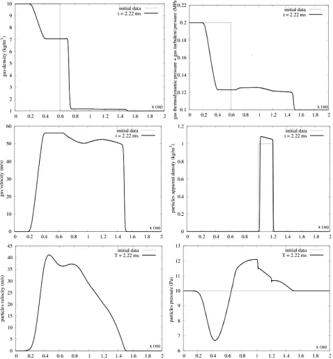
A shock wave propagates to the right in the gas phase while a rarefaction wave propagates to the left. The shock then interacts with the particle cloud and a diffrac-tion phenomenon occurs. A shock is transmitted to the cloud and a weak reflected shock is emitted to the left from the cloud interface. The particle cloud compresses and moves to the right. The various flow variables pro-files are shown in the Figure 3 at time 2.22 ms.

We now examine the turbulent model numerical solu-tion in the same configurasolu-tion.

 Turbulent model results

With th lent model the initial turbulent pressures have to be set. We set for both phases a weak initial pressure of 10 Pa. The turbulent viscosity is arbitrarily

3

2.10

 _ 

t to t kg/m/s. In the one-dimensional case,

the value of this parameter has no influence as will be shown later. The flow variables profiles are shown at the same time (t = 2.22 ms) in the Figure 4.

The weak particles volume fraction ( ₁₀6

p

 _  _{) on}

both sides of the cloud implies a fast acceleration of the particles outside the cloud (see the particles velocity graph of Figure 4), but the small particles proportion has no influence on the gas motion.

The particle velocity profiles of Figures 3 and 4 have me

so differences, but these diff sid

erences are located

out-comparison, we sh

ined hereafter the influ-en

e the cloud, where the particles are absent. So, these differences have no importance. For the same reason turbulent pressure profiles must be observed within the cloud.

Figures 3 and 4 show the same behavior for gas

ve-locity, pressure and density. The apparent particles den-sity profiles also are closed. For a better

ow the particles variables in the particles cloud only and on the same graphs in the Figure 5.

Excellent agreement is observed between the two computations, showing that in one dimension, the two models are equivalent. We exam

ce of the turbulent viscosity parameter. 8.1.2. Influence of Turbulent Viscosity

We now consider the turbulent model only and use dif-ferent values of the turbulent viscosity: 3 0 2.10

t

 _ _ 

kg/m/s, t 100 and t 1000. The apparent par-ticles density and the parpar-ticles velocity profiles are plot on the same graph for each value of the turbulent viscos-ity. Corresponding results are shown in the Figure 6.

For this 1D test problem, it appears clearly that the turbulent viscosity has no influence on the cloud dynam-ics. In all these computations, the initial turbulent pres-sure was set to 10 Pa. We now investigate the influence of this initial condition to the results.

.1.3. Influence of the Initial Turbulent Pr

8 essure

urbulent pres-We now consider three different initial t

sures (Pt10 Pa , Pt 50 Pa, Pt 250 Pa) for the

same two-phase shock tube test. The turbul is set to

ent viscosity 0

 . Correspondin ults are shown in the Figure 7 at time t = 8.6 ms.

Some influence appears, in particular a dissymmetry in the cloud, due to the fact that the turbulent pressure pr

g res

ncouraging as the in figuration

oduction is different on the left and the right sides of the cloud. These differences are not significant enough to detect unphysical behavior.

In the one-dimensional case, whatever the turbulent parameters are, the two models (pressureless and

turbu-nt) yield very closed results. This is e le

pressureless model is considered as quite accurate such flow conditions. We now examine two-dimensional flow con s.

8.2. Two-Dimensional Configurations

We now consider a more sophisticated situation where extra effects appear. It consists in the injection of a parti-

S. HANK ET AL. 1004

Figure 3. Gas and particles variables profiles at times t = 0 and t = 2.22 ms for the two phase shock tube test case with the conventional pressureless model.

cle jet in air at rest. In order to exclude the effects of dy-namics fragmentation with liquid jets, that contain extra physics, we consider solid particles jets. Careful experi-mental studies were done independently [13,14] with particles made of different materials. Corresponding ex-perimental data will be used for model's validation. Both experimental configurations can be summarized as

shown in the Figure 8. A particle injector of a few mil-limeters diameter is used to inject a free particle jet into an open cavity initially filled with air at atmospheric conditions.

In [13,14] experiments, cross cut of apparent density profiles are given at various locations from the injecto (C1, C2, C3). The configurations used by these authors

Figure 4. Gas and particles variables profiles at times t = 0 and t = 2.22 ms for the two phase shock tube test case with the new turbulent model.

are reported in the Table 1.

To deal with numerical simulations of corresponding test problems, initial and boundary conditions as well as flow model parameters have to be specified.

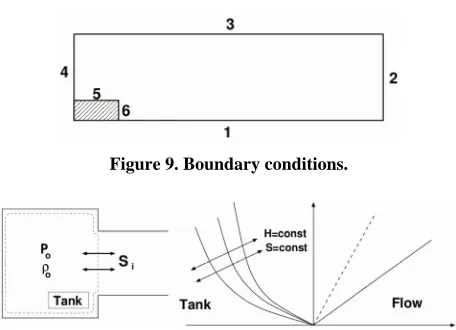
8.2.1. Boundary Conditions

The computational domain contains 6 different bounda-

ries shown in Figure 9.

1006 S. HANK ET AL.

Figure 5. Comparison of pressureless and turbulent models solutions on the shock tube test problem. Apparent density and velocity profiles are in perfect agreement.

Table 1. Experimental data for solid particle jet injection in air from [13,14].

[14] [13] Particle diameter ( m)　 500 64

Material density (kg/m3_{) 1020 2590}

Injection speed (m/s) 24 30

Injection apparent density (kg/m3_{) 0.2 1.0}

Injector diameter D (mm) 20 13

responds to a supersonic particles injection with respect to the turbulent speed of sound. Thus all data of the Ta-ble 1 are imposed at this boundary. Boundary 4 is treated as a tank for both gas and particle phases. Numerica

ystem (11),

8.2.2. Gas Phase

The ste ons redu :

l treatment of this specific boundary needs particular care. Part of the solution is obtained by assuming a steady flow between the tank and the inlet section. S

in the stationary case is integrated in a control volume which is represented to the left of Figure 10.

ady gas phase equati ce to

Figure 6. Influence of the turbulent viscosity on the shock tube test case results. The apparent particles density as well as the particles velocity in the particle cloud shows no in-fluence. The results are compared at time t = 8.6 ms.

0 ( ) 0

( ( ) )

( ( ) ) 0

( ) 0

t t t

u

u u P P I Eu P P u us

   

 



    



   



 

   

 



u n  Using the slip condition on the lateral surfaces ( = 0), the integration of the mass equation gives (variables with subscript i, corresponds to variables at the inlet sur-face, those with subscript 0 corresponds to tank vari-ables):

0 0

(uS)i(uS)  (12) This relation is undetermined, indeed and

. Nevertheless it can be used

turbulent entropy equations. Fo en 0

S   to integrate the

en-r the total

0 0

u 

ergy and -

ergy, the integration gives, with the help of (12),



 



2

u P

where,

2

H e t

t t

P h e 

  and 



Figure 7. Influence of the turbulent initial pressure in the dispersed phase. The particles apparent density and veloc-ity profiles in the particles cloud are shown at time t = 8.6 ms for three initial pressures.

Figure 8. Schematic representation of the experimental fa- cility of [13,14] for solid particles jets injection in air.

A first relation is thus available to solve the boundary Riemann problem. The momentum conservation equa- tion cannot be integrated as the pressure integral is un-known on the lateral surface. Integration of turbulent entropy equation using (12) results in:

0

ti t

s s (14) It is the second available

Figure 9. Boundary conditions.

Figure 10. Schematic representation of the tank boundary condition.

equation is required to close the full system. This one corresponds to thermodynamic

tween the tank and the inlet section, e

entropy conservation be- xpressed as:

0

i

P P

   

 

  

   

    (15) Then a Riemann solver is built where the left facing wave jump conditions (Riemann invariants or shock re-lations) are replaced by System (13-15). The right facing

wave obeys t l as the

con-tact discontinui 8.2.3. Particle Phase

In the same way, the system associated to the particle phase is integrated in the control volume. The stationary system reads:

0 o conventional relations, as wel

ty.

( ) 0

( )

( )

p p p pt

u

u u P I E u P u 



 



0

p p

 

( ) 0

p p p pt p

p p ptu s



   



  



 

   

 



Following the same methodology, the following rela-tions are obtained:

0 0 (p pu S)i(p pu S) 

 

(16) 0

( )e_{p i} ( )e_p (17) 0

(Hpt i) (Hpt) (18)

0

t t

pt pt

p _i p

P P

   

_  _ _  _

    (19)

with

2

2

pt

pt pt

p

P u

H e



   .

S. HANK ET AL. 1008

jump conditions are replaced by System (17-19). 8.2.4. Initial Conditions

The gas is initially at rest under atmospheric conditions with a low turbulent pressure = 10 Pa). The particles have an initial non-zero vol fraction in the entire do

(Pt

ume

main, corresponding to the apparent density of ₁₀3 3

kg/m , associated to a volu fraction of the . Initial turbulent pressure the

e value as in gas phase ( me

of

order of 6

10

the sam

particles is set to

pt

P = 10 Pa). 8.2.5. Model Parameters

The same drag force correlation (

viscosity is used as in the preceding 1D example kg/m/s). In all compu

viscosity is constant and equal to

7) with the same gas ( _19.106

g

 _ 

lent

tations, the turbu-3

2.510 t

 _ 

kg/m/s.

8.2.6. Qualitative Compari ons s Th

ectories cor-to straight lines. With the turbulent model, jet preading occurs.

own in the Fig-ur

with the Experimental Data of [14] he same computations are done for the configuration lent one are shown in the Figure 11.

Large differences between the two computed jets are clearly visible. With the pressureless conventional model, no jet enlargement occurs. The particles traj

respond s

8.2.7. Comparison with the Experimental Data of [13] A computational domain involving 280 × 100 cells is used on the geometrical configuration sh

e 8 with parameters given in the Table 1. The normal-ized apparent density profiles are shown in the Figure 12 and compared with experimental data at steady state. 8.2.8. Comparison

T

reported in [14]. The normalized apparent density pro-files at steady sate are shown in the Figure 13 and com- pared to experimental.

In this case too, the results obtained with the turbulent model and the experimental data are in a very good e particle jet dynamics computed alternatively with

the conventional pressureless model and the new

Figure 12. Computed results in lines versus experimental data of [13]. Normalized apparent density  _p/ _p0

30 D. to collisi

y the mod noted by

Figure 13. Computed results in lines versus experimental data of [14]. Normalized apparent density

cross cut at

abscissa C1 = 10 D, C2 = 20 D and C3 = The jet width

increases during its propagation, due onal turbulent

effects that are perfectly reproduced b el. The

ap-parent density along the centerline is de _p0.

0

/  _{p p} 10 D and C3 = 15 D. The jet

o co uced b rline is de

cross cut at abscissa C1 = 4 D, C2 =

width increases during its propagation, due t llisional

turbulent effects that are perfectly reprod y the

model. The apparent density along the cente noted

by p0.

agreement. For the last graph of Figure 13 the agreement is not as good as for the other graphs. But it can be no- ticed on the experimental curve that some noise is pre- sent. The experimental cross cut of the apparent particle density contains oscillations. It means that an error bar is

present in the experiments. Also, the variable plot on this graph corresponds to the normalized density  p/ p₀.

1010 S. HANK ET AL.

Figure 14. Results comparison with the different models on the configuration studied in [14].

become small. Thus, the ratio  p/ p0 becomes inac-curate.

The results of Figures 13 and 14 are obtained with the same turbulent viscosity of kg/m/s. This agree-ment is particularly interesting as t e experiagree-ments of [13] and [14] deal with very different materials density, dif-ferent particles diameter and injector diameters.

When the same computations are done with the

pres-sureless model (1-2), no jet enlargement appears, as shown in the Figure 14. The same remark holds when the turbulent viscosity is set to zero in the new model.

Consequently the new model admits the same solution as the pressureless equations in the limit of vanishing turbulent viscosity and is able to improve considerably the predictions and capabilities with non-zero turbulent viscosity.

9. Conclusions

A new two-phase flow model for dilute particles suspen-sions has been developed. Compared to conventional pressureless particle dynamic models the new one is

n s cessfully reproduced by the model with the same turbulent viscosity coefficient, of the order of

3 2.10

h

strictly hyperbolic. It also has enhanced physical capa-bilities, thanks to a simple modeling of particles colli-sions. Indeed, turbulence production in the new model is linked to a turbulent viscosity, aimed to mimic particles collisions. Particles jets dispersion experiments from different authors and under different configurations have bee uc

3

2.10 _{kg/m/s, while the experimental conditions}

(parti-cles diameter, parti(parti-cles density and injector diam e varying considerably.

eter) ar

10. References

[1] F. E. Marble, “Dynamics of Dusty Gases,” Annual Re-view of Fluid Mechanics, Vol. 2, No. 1, 1970, pp. 397-446. doi:10.1146/annurev.fl.02.010170.002145 [2] Y. B. Zeldovich, “Gravitational Instability: An

Approxi-mate Theory for Large Density Perturbations,” Astron & Astrophys, Vol. 5, No. 84, 1970, pp. 168.

[3] P. D. Lax, “Weak Solutions of Nonlinear Hyperbolic Equations and Their Numerical Computation,” Commu-nications on Pure and Applied Mathematics, Vol. 7, No. 1, 1954, pp. 159-193.

[4] R. Saurel, E. Daniel and C. Loraud, “Two-Phase Flows: Second-Order Schemes and Boundary Conditions,” AIAA Journal, Vol. 32, No. 6, 1994, pp. 1214-1221.

doi:10.2514/3.12122

[5] Y. Brenier and E Grenier, “Sticky Particles and Scalar Conservation Laws,” SIAM Journal on Numerical Analy-sis, Vol. 35, No. 6, 1998, pp. 2317-2328.

doi:10.1137/S0036142997317353

[6] A. Chertock, A. Kurganov and Y. Rykov, “A New Sticky Particle Method for Pressureless Gas Dynamics,” SIAM Journal on Numerical Analysis, Vol. 45, No. 6, 2007, pp. 2408-2441. doi:10.1137/050644124

[7] R. Saurel, S. Gavrilyuk and F. Renaud, “A Multiphase Model with Internal Degrees of Freedom: Application to Shock-Bubble Interaction,” Journal of Fluid Mechanics, Vol. 495, No. 1, 2003, pp. 283-321.

[8] G. Rudinger, “Some Effects of Finite Particle Volume on the Dynamics of Gas-Particle Mixtures (Gas Particle Mixture with Finite Particle Volume Affecting Frozen and Equilibrium Flows Behind Shock Wave),” AIAA Journal, Vol. 3, 1965, pp. 1217-1222.

[9] R. Saurel, A. Chinnayya and F. Renaud, “Thermody-namic Analysis and Numerical Resolution of a Turbu-lent-Fully Ionized Plasma Flow Model,” Shock Wa

Vol. 13, No. 4, 2004, pp. 283-297. doi:10.1007/s00193-003-0216-z

ves,

[10] E. F. Toro, “Riemann Solvers and Numerical Methods for Fluid Dynamics: A Practical Introduction,” Springer Ver-lag, Berlin, 1997.

[11] L. Schiller and Z. Naumann, “A Drag Coefficient

Corre-lation,” VDI Zeitung, Vol. 77, 1935, pp. 318-320. [12] E. F. Toro, M. Spruce and W. Speares, “Restoration of

the Contact Surface in the HLL-Riemann Solver,” Shock Waves, Vol. 4, No. 1, 1994, pp. 25-34.

doi:10.1007/BF01414629

[13] K. Hishida, K. Kaneko and M. Maeda, “Turbulence Structure of a Gas-Solid Two-Phase Circular Jet,” Trans. JSME, Vol. 51, 1985, pp. 2330-2337.

doi:10.1299/kikaib.51.2330

[14] Y. Tsuji, Y. Morikawa, T. Tanaka, K. Karimine and S. Nishida, “Measurement of an Axisymmetric Jet Laden with Coarse Particles,” International Journal of Multi-phase Flow, Vol. 14, No. 5, 1988, pp. 565-574.

doi:10.1016/0301-9322(88)90058-4

s

A. Numerical method for diffusive term

Time explicit integration of corresponding terms is con-sidered:

 

 (  )d d   ( ) d

i t p t p

t V u V t t S u n S



 



( )d d ( )d

i

T T

t p p t p p

t V u u V t t Su u n S

      

 



Space integration is detailed in 1D, multi-D extension being simi



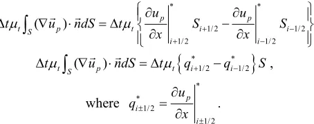
lar. The space integration is transformed suc-cessively as,

* *

1/ 2 1/ 2

1/ 2 1/ 2

( )

t _S p t i i

i i

t u ndS t S S

x x

  _{ }

 

     _  _

 

 

 







1/ 2 1/ 2

( )

t _S p t i i

t u ndS t q q S



_

where

p p

u u

 



  

* *

1/ 2

1/ 2

p i

i u q

x 



 

 .

Two neighboring computational cells i and i + 1, sepa-rated by cell boundary i + 1/2 are schematized in the Figure 15. The velocity derivative q*i1/ 2 has precisely to be expressed at these cell boundaries.

following intercell conditions are used:

* * *

u u u

q q

_  _

The

*

ts (–) and (+) denotes respectively *_ *_q

where the superscrip

* *

1 1 2 1 2

* * ui ui ui ui

2 2

q q

x x

 

  

  ,

* 1

1/ 2

2 i

u i i

u u



The cell boundary velocity derivative reads conse-quently,

* 1

1/ 2 i i

i

u u

q

x

 

 

 ,

* 1

1/ 2 i i

i

u u

q

x

 

 



In the one-dimensional case, viscous derivative terms are thus approximated by:

1 2 1

( ) d i i i

t _S p t

u u u

t u n S t S

x

     

    





2 2 2

1 2 1

( )d

2

T i i i

t _S p p t

t u u n S t S

x

 

    



