Stability of Stochastic Logistic Model with Ornstein Uhlenbeck Process for Cell Growth of Microorganism in Fermentation Process

ISSN Online: 2152-7393 ISSN Print: 2152-7385

DOI: 10.4236/am.2019.108047 Aug. 13, 2019 659 Applied Mathematics

Stability of Stochastic Logistic Model with

Ornstein-Uhlenbeck Process for Cell Growth of

Microorganism in Fermentation Process

Tawfiqullah Ayoubi

School of Mathematics and Statistics, Southwest University, Chongqing, China

Abstract

Current research is concerned with the stability of stochastic logistic equation with Ornstein-Uhlenbeck process. First, this research proves that the stochas-tic logisstochas-tic model with Ornstein-Uhlenbeck process has a positive solution. After that, it also introduces the sufficient conditions for stochastically stabil-ity of stochastic logistic model for cell growth of microorganism in fermenta-tion process for positive equilibrium point by using Lyapunov funcfermenta-tion. In addition, this research establishes the sufficient conditions for zero solution as mentioned in Appendix A due to the cell growth of microorganism µmax, which cannot be negative in fermentation process. Furthermore, for numeri-cal simulation, current research uses the 4-stage stochastic Runge-Kutta (SRK4) method to show the reality of the results.

Keywords

Stability, Fermentation Process, Ornstein-Uhlenbeck Process, Logistic Model, Lyapunov Function, 4-Stage Stochastic Runge-Kutta Method

1. Introduction

Stochastic differential equations (SDEs) have been intensively used to model the natural phenomena in the last decades and these equations play a prominent ap-plied role in various fields [1] [2]. Most SDEs do not have explicit solution but these equations can be solved numerically to approximate their solutions [3]. We use the SRK method to approximate the solution numerically ([3], p. 69) [4] [5] [6] [7]. Whereas, Rüemelin in [8] proposed the S-stage stochastic Runge-Kutta explicit method. Moreover, Xiao in [9] introduced the High strong order sto-chastic Runge-Kutta methods for stosto-chastic differential equations in case of How to cite this paper: Ayoubi, T. (2019)

Stability of Stochastic Logistic Model with Ornstein-Uhlenbeck Process for Cell Growth of Microorganism in Fermentation Process. Applied Mathematics, 10, 659-675. https://doi.org/10.4236/am.2019.108047

Received: July 2, 2019 Accepted: August 10, 2019 Published: August 13, 2019

Copyright © 2019 by author(s) and Scientific Research Publishing Inc. This work is licensed under the Creative Commons Attribution International License (CC BY 4.0).

http://creativecommons.org/licenses/by/4.0/

DOI: 10.4236/am.2019.108047 660 Applied Mathematics Stratonovich since our model is in Stratonovich sense.

This research deals with the stability of stochastic logistic model with Ornstein-Uhlenbeck process. This process is a batter model of Brownian motion ([10], p. 86). The Ornstein-Uhlenbeck process is used to model stock price, cur-rency exchange rates and velocity.

The classical Brownian motion was introduced by Scottish Botanist Robert Brown in (1827). He described this motion based on random movements of pol-len grains in liquid or gas [11]. This theory was further supported by Norbert Wiener (1923) who explained full mathematical theory of Brownian motion which existed as a rigorously defined mathematical objective to recognize his contribu-tion [12]. Brownian motion is a simple continuous stochastic process which is extensively used to model phenomena in various fields such as industry, dynam-ic process, physdynam-ics, finance and fermentation process [3] [11] [12]. This Brow-nian motion is the cause of instability (turbulence) in fermentation process [1].

Fermentation process converts sugar into alcohol with the help of yeast [13]. Ma-dihah, in [14] used the logistic model to elaborate the cell growth of Clostridium acetobutylicum p. 262 in fermentation process proposed by Verhulst (1838). This model is inadequate to describe the cell growth of microorganism in fermentation process because fermentation process contains random fluctuations. Bahar and Mao in [2] introduced new stochastic logistic model for population dynamics. The sto-chastic logistic model was used in [15] to elucidate the cell growth of Clostridium acetobutylicum p. 262 in fermentation process. This cell growth of microorganism in fermentation process is affected by environmental noise, a batter model for model-ling environmental noise is Ornstein-Uhlenbeck process. However, no specific re-search was conducted on stability stochastic logistic model with Ornstein-Uhlenbeck process for cell growth of microorganism in fermentation process. Nevertheless, there are some previous research works which have been done on stability of logis-tic equations with white noise, Lévy Jumps and other different aspects [16]-[22]. None of these researches were investigated the stability of stochastic logistic model with Ornstein-Uhlenbeck process for cell growth of microorganism in fermenta-tion process. This research establishes the sufficient condifermenta-tions for stochastic logis-tic equation with Ornstein-Uhlenbeck process for positive equilibrium point and zero solution by using Lyapunov function. Since, the Ornstein-Uhlenbeck process is a better model of Brwonian motion ([10], p. 86). In addition, our current study will indicate that the Ornstein-Uhlenbeck process is unfavorable for stability of cell growth in fermentation process. Moreover, we apply the SRK4 method to evaluate the numerical solution.

This paper is organized in five main sections; Introduction, Preliminaries and Models Description, Main Results, Numerical Simulation and Conclusion.

2. Preliminaries and Models Description

Throughout this paper; the notation E x t_

( )

_{ is the expectation of}

(

x t

( )

)

, T

maxi-DOI: 10.4236/am.2019.108047 661 Applied Mathematics mum specific growth rate, xmax illustrates a carrying capacity,

σ

indicates the random fluctuation, W t

( )

shows Brownian motion and b is a constant.

The simplest mathematical model to illustrate the exponential phase for cell growth in fermentation process is:

( )

_{( )}

max

d

. d

x t

x t

t =µ × (1)

The solution of Equation (1) is:

( )

max

0et ,

x t ₌x ×µ ₍₂₎

where t is time, x0 corresponds to the initial cell size and µmax denotes the maximum specific growth rate. If µmax >0, Equation (1) is strongly ascending, and if, µmax <0, strongly descending. Hence, Equation (1) is not adequate to model stationary phase in fermentation. Therefore, Pierre Francois Verhulst (1838) introduced new model containing stationary phase in fermentation process. Thus, the exponential growth model (1) is augmented by the inclusion of multiplicative factor of

( )

max

1 x t

x

− _{. Hence, the logistic ordinary differential equation is:}

( )

max

( ) ( )

max

dx t 1 x t x t td ,

x

µ  

=  − 

  (3)

where xmax is a carrying capacity of a microbial species and Equation (3) can be solved analytically by determining the solution is:

( )

(

)

max

max

max 0 max 0

e _, 1 e

t

t x x

x t

x x

µ

µ =

+ − + (4)

where x t

( )

is the highest cell size. Madihah, in [14] used Equation (3) to ela-borate cell growth of Clostridium acetobutylicum p. 262 in batch fermentation process. Murray in [23] and May in [24] were proved that Equation (3) is stable. This model is inadequate to describe the cell growth of Clostridium acetobutyli-cum p. 262 in fermentation process because fermentation process suffers from random fluctuation. Bahar and Mao in [2] introduced new stochastic logistic equation to model uncontrolled fluctuation in stationary phase at fermentation process by using new perturbation very randomly which is:

( )

d , d

W t t

ρ→ +ρ σ ₍₅₎

where max

max

x µ

ρ = _{is diffusion coefficient. Model (3) with perturbation (5) is:}

( )

( ) ( )

2

( )

( )

[ ]

max

max

dx t 1 x t x t td x t W t td , 0, ,T x

µ   σ

=  −  + ∈

  (6)

where W t

( )

is m-dimensional Weiner process and

σ

is corresponding to the random fluctuation. Bazli, in [15] used Equation (6) to evaluate the cell growth of Clostridium acetobutylicum p. 262 in fermentation process.

DOI: 10.4236/am.2019.108047 662 Applied Mathematics white noise which cannot model random fluctuations in stationary phase. There-fore, this research introduces new stochastic logistic model to cope with this prob-lem and established the sufficient condition for positive equilibrium point. The new model is Equation (6) with Ornstein-Uhlenbeck process. The Ornstein-Uhlenbeck process is:

( )

( )

d

( )

y t′′ = −by t′ + W t (7)

where y t

( )

stands for positive Brownian motion at time t, b>0 _{shows the}

coefficient friction,

σ

indicates the diffusion coefficient and W t

( )

is white noise.

By substituting

( )

( )

,

y t′ =W t (8) into Equation (7) hence, the Ornstein-Uhlenbeck process becomes;

( )

( )

( )

dW t = −bW t td +σdW t . (9)

Substituting Equation (9) into Equation (6) yields

( )

( ) ( )

2

( )

( )

2

( )

2

( )

max

max

dx t 1 x t x t td x t bW t t x td dW t .

x

µ   σ σ

= _ − _ − +

  (10)

Equation (10) is stochastic logistic model with Ornstein-Uhlenbeck process. 

3. Main Results

First, it is needed to prove that Equation (10) has a unique positive solution and later on we will pay attention on stability.

Theorem 3.1: For all t≥0 and for any 0<x

( )

0 =x0 Equation (10) has a unique positive solution.

Proof: For any given initial value x0∈R+n, the coefficients of Equation (10) are locally Lipschitz continuous. Hence, there is a unique locally solution

( )

,

[

0,e

)

x t t∈ i Where ie shows the explosion time Arnold in [25] and Friedman

[26]. To show that the x t t

( )

, ∈

[

0,ie

)

is a unique positive solution. So, it is

really necessary to determine that ie→ ∞. Let 0 0 0 0

1 , , 0

k k k

k

 

∈_{ } >

  and k k> 0 is sufficiently large for each component of x0, the stopping time for every in-teger k k> 0 is:

[

) ( )

1

inf 0, : is not in , .

k e

t t i x t k

k

  

=  ∈ _ _

 

0

k is sufficiently large means that the tk is increasing as k→ ∞. Hence, limk k

t∞ = →∞t , whereas t∞ ≤ie.

If we can show that i∞ = ∞ a.s., then i∞ = ∞ a.s. and x t

( )

∈R+n a.s. for all

0

t≥ _{. In other words, to complete the proof all we need to show is that} i∞ = ∞ a.s. For if this statement is false, then there is a pair of constants T >0 and

( )

0,1

∈

 such that

{

}

.

DOI: 10.4236/am.2019.108047 663 Applied Mathematics Therefore, there exist an integer k1≥k0

{

}

, 1

P i∞ ≤T ≥ ∀ ≥ k k (11)

Define

(

( )

)

( )

1 1ln

( )

2

V x t =_ x t − − x t _

  for all x t

( )

∈

[

0,ie

)

and the

nonne-gativity of this function can be seen from

1 1 ln

2

u− − u

Itô ([27], p. 95) [28] [29] [30] ([31], p. 54) formula shows that

( )

(

)

(

)

_{( )}

_{( )}

( ) ( )

( )

( )

( )

( )

( )

( )

( ) ( )

( )

( )

( )

( )

max max

2 2 2

max 2

3

max 2

2 2 2

1 1

d 1 d

2 2

d d

0.25 1

0.5 1 d

2 d d A A B B x t

V x t x t t

x t x

x t

x t bW t t x t W t

x t

x t t x

x t x t

x t bW t t x t W t

µ σ σ µ σ σ     = −   −           −_ + _  _{   }  + − _  −  _  _{   }   − + _      (12)

To simplify A and B separately yields

( )

( ) ( )

( )

( )

( )

( )

( )

( )

( )

( ) ( )

( )

( )

( )

( )

( )

( )

2 max max 2 2 max max

2 2 2

1 _{1 d} 1 _d

2 2

1 _d 1 _{1 d}

2 2

1 _d 1 _d

2 2

x t

A x t t x t bW t t

x

x t x t

x t

x t W t x t t

x t x

x t

x t bW t t x t W t

x t x t

µ σ σ µ σ σ   =  −  −     + −  −    + −

( )

( )

( ) ( )

( ) ( )

(

( )

( )

( )

( )

)

( )

( )

( )

( )

(

)

2 max 2 3 max

2 2 2

max

max

2

2 2 2

0.25 1 _{1 d} 2

2 1 d d d

d d

x t

B x t t

x x t

x t

x t

x t t x t bW t t x t W t

x

x t bW t t x t W t

µ

µ σ σ

σ σ      = − _  −  _ _{   }      + _  −  _ − +      + − +  

( )

( )

( )

( )

( )

( )

( )

( )

( )

( )

( )

(

)

(

( )

( )

)

( )

( )

(

)

(

( )

( )

)

(

( )

( )

)

2

2 2 max 2

max 2 3 max 2 2 max max max max max 2

2 2 2 2

2

2 2 2 2 2

0.25 1 _{d d 2 d d}

2

d 2 d d

d d d

2 d d d

B x t t t x t t t

x x t

x t

x t t x t t x t t

x x

x t bW t t x t W t x t bW t t

x t bW t t x t W t x t W t

µ µ

µ µ

µ

σ σ σ

σ σ σ

DOI: 10.4236/am.2019.108047 664 Applied Mathematics An application of these facts d dt× =t 0,d dt× w t

( )

=0 _and dW t

( )

×dW t

( )

=dt

([32], p. 87) and somewhat lengthy calculation we have

( )

2

( )

(

4 4

( )

)

3

0.125 0.25 _d

B x t t

x t

x t σ

= −

( )

( )

( )

( )

4 4 4 4

2 3

0.125 x t td 0.25 x t td

B

x t x t

σ

σ

⇒ = −

By substituting the value of A and B into Equation (12) yields

( )

(

)

(

)

( )

( ) ( )

( )

( )

( )

( )

( )

( )

( )

( )

( )

( )

( )

( )

( )

( )

( )

( )

2 max max 2 2 max max 2

4 4 4 4

2 3

1 1

d 1 d d

2 2

1 _d 1 _{1 d}

2 2

0.5 d 0.5 d

0.125 d 0.25 d

x t

V x t x t t x t bW t t

x

x t x t

x t

x t W t t

x t x

x t

x t bW t t x t W t

x t t x t t

x t x t µ σ σ µ σ σ σ σ  _{ }  =  −  −  _{ }    + − _ − _    + − _  + − (13)

( )

(

)

(

)

( )

( )

( )

( )

( )

( )

( )

( )

( )

( )

( )

( )

( )

( )

0.5 0.5 max max max max 4 2.5

4 2 2 2 2

d 0.5 1 0.5 1

0.5 0.5 0.125

0.125 d 0.5 d d 0.5 d

x t x t

V x t x t x t

x x

x t bW t x t bW t x t

x t t x t W t t x t W t

µ µ

σ σ σ

σ σ σ

−      =  − −  −        − + +  − _ − −  (14)

( )

(

)

(

)

( )

( )

( )

( )

( )

( )

(

( )( )

)

(

( )

)

( )

( )

(

( )

)

0.5 0.5 max max max max

0.5 4 2

2 0.5

d 0.5 1 0.5 1

0.5 1 0.25 0.5 1 d 0.5 d 1

x t x t

V x t x t x t

x x

x t bW t x t t x x t t

x t W t x t

µ µ σ σ σ −      =  − −  −         + − + _{− }  + − (15) Worth mentioning,

( )

( )

( )

( )

( )

(

)

0.5 0.5 max max max max 4 2

0.5 1 0.5 1

0.25 0.5 1

x t x t

x t x t

x x

x x t

µ µ σ −     − − −         + − (16)

( )

( )

( )

( )

( )

(

( )

)

0.5 0.5 max max max max 4 2

0.5 1 0.5 1

0.25sup 0.5 1 .

t R

x t x t

x t x t

x x

x t x t

µ µ σ ∨ ∨ + − ∈     ≤ _ − _− _ − _     + − (17)

If x t

( )

≤xmax then

( )

max

1 x t 0

x

 

− ≥

 

  , it follows the boundedness

σ

. Therefore, there is nonnegative number Q1 which independent of x and t.

inde-DOI: 10.4236/am.2019.108047 665 Applied Mathematics pendent of x and t, and it follow bounded

σ

, such that

( )

( )

( )

( )

( )

(

)

( )

( )

( )

( )

( )

(

)

0.5 0.5

max max

max max

4 2

0.5 0.5

max max

max max

4 2

2

0.5 1 0.5 1

0.25 0.5 1

ˆ ˆ

0.5 1 0.5 1

0.25sup 0.5 1 .

t R

x t x t

x t x t

x x

x x t

x t x t

x t x t

x x

x x t Q

µ µ

σ

µ µ

σ

+

−

−

∈

   

− − −

   

   

+ −

   

≤ _ − _− _ − _

   

+ − ≤

(18)

On the other hand, we show that there is a nonnegative number Q which inde-pendent of x and t such that

( )

( )

( )

( )

( )

(

)

0.5 0.5

max max

max max

4 2

0.5 1 0.5 1

0.25 0.5 1 .

x t x t

x t x t

x x

x x t Q

µ µ

σ

−

   

− − − −

   

   

+ − ≤

(19)

By substituting the inequality (19) into Equation (13) yields

( )

(

)

(

)

( )

( )

(

( )( )

)

( )

( )

(

( )

)

0.5

2 0.5

d d 0.5 1 d

0.5 d 1 .

V x t Q t x t bW t x t t t

x t W t x t

σ σ

≤ + −

+ − (20)

where W t

( )

is Brownian motion, and taking integral and expectation

(

)

(

)

(

n

)

(

( )

0

)

(

n

)

(

( )

0

)

.

E V x i T∧ ≤V x +QE i T∧ ≤V x +QT (21)

By taking into account, the inequality (11) then we have

(

n

)

.

P i ≤T ≥

For every ∈

(

in≤T

)

, x i

(

n,ω =

)

n or

( )

i,ω =1_n. Therefore, V x t

(

( )

)

is no

less than either

( )

( )

1 1 1

min 1 ln , 1 ln .

2 2

k k k

k

 

− − − +

 

 

Based on (20) we have

( )

(

)

{

}( )

(

( )

)

( )

( )

0

1 1 1 min 1 ln , 1 ln .

2 2

n n

V x QT E i T V x i

k k k

k

ω

 

+ ≥ _ ≤ _

 

≥ _ − − − + _

 



where

{

in ≤T

}( )

ω illustrates the function

{

in ≤T

}

. Letting n tends to infinity

leads to dissidence

( )

(

0

)

V x QT

∞ > + = ∞

Therefore, we need to have i∞ = ∞. Eventually, our claim is proved truly.  In the next section we prove that Equation (10) with Ornstein-Uhlenbeck process is globally asymptotically stable in positive solution which illustrates the highly randomness in stationary phase.

equi-DOI: 10.4236/am.2019.108047 666 Applied Mathematics librium points xmax, under following assumptions a.s.

H1: For

1) 0≤t0, 0<x0< <σ µmax < <b xmax 2) 0≤t0, 0<x0< < <σ b xmax <µmax and the

( )

( )

0 d 0 d ˆ

limsup and liminf .

t t

t t

x s s x s s

b b t t ∨ →∞ →∞ = =

∫

∫

where, b∨ and bˆ are positive constant then the solution x t

( )

satisfies the

( )

max

limt→∞x t =x .

Proof: An application Itô’s formula ([27], p. 95) [28] [29] [30] for Equation (10) and somewhat lengthy calculation leads to

( )

( ) ( )

( )

( )

(

)

( )

( )

max 2

0 _{0 0}

4 2

max max

max

0 0 0

max 0

1 exp d d

1

exp d d d 1

2

t t

t t t

x x t

x b x s W s s x s W s

x

x s s x s s s

x x

σ σ

µ σ _µ

=  +_ +  ×  _{− − −}   −       

∫

∫

∫

∫

∫

(22)

For the convenience we set the denominator of Equation (22) to

Q

and ac-cording to the ([10], p. 69), we have:

( ) ( ) ( ) ( ) ( )

( ) ( ) ( )

max max

0 _max 0 0 0

2 4 2

0 0

d d d d

1

d d

2

1 e

e .

t t t t

t t

s x s s bW s W s x s W s x

x s W s x s s Q µ µ σ σ σ _{− − − ×}         ₋      ∫ ∫ ∫ ∫ ∫ ∫ = + ×

Taking limit from both sides of above equation yields:

( ) ( ) ( ) ( ) ( ) ( )

( ) ( ) ( ) ( )

max

0 max 0 0 0

max

2

20 40

d d d d

d 1 d

2

lim 1 lime

lime .

t t t t

t t

s x s s bW s W s x s W s t

t x t t t

t t

x s W s x s s t

t t

t

Q

µ µ σ

σ σ   − + +   →∞ →∞   − − +   →∞ ∫ ∫ ∫ ∫ ∫ ∫ = + × (23) where,

( )

( )

( )

0 d t

x s W s =M t

∫

(24)

is a Martingale with quadratic variation

( ) ( )

2

( ) ( )

0

, t d

M t M t =

_∫

x s s ₍₂₅₎

Based on ([31], p. 65) the

( )

limsup 0 . .

t

M t

a s t

→∞ = (26)

and

( ) ( )

,

limsup . .

t

M t M t

C a s t

DOI: 10.4236/am.2019.108047 667 Applied Mathematics where C R_∈ + _{then Equation (23) becomes}

( ) 0 max max 0 ( ) 4 max

d d 1

2

lim 1 lime

t _s t_{x s s}

t C

t x t

t Q t

µ µ _σ

 

 

− _ + + _

 

 

→∞ →∞

∫ ∫

= + ₍₂₈₎

( ) 0 max max 0 ( ) 4 max

d d 1

2

lim 1 lime 0 . .

t _s t_{x s s}

t C

t x t

t Q t a s

µ µ _σ

 

 

− _ + + _

 

 

→∞ →∞

∫ ∫

= + = ₍₂₉₎

By substituting Equation (29) into Equation (22) we have:

( )

max

lim lim

t→∞x t =t→∞x

( )

max

lim .

t→∞x t x

⇒ =

Ultimately, prove is completed. 

Remark 3.1: Liu et al., in [21] studied the stability of stochastic logistic model with white noise which illustrates highly randomness in lag phase and the sta-tionary phase is steady means there is no fluctuations. In lag phase microbes are adapted with each other and as a result no growth takes place. But, the model, con-ditions and approach which are presented in this study quite different and easy respectively. This research considers Equation (6) with Ornstein-Uhlenbeck process which highly presents the randomness in stationary phase. In stationary phase microbes fight with each other to survive (uncontrolled fluctuations reached max-imum level). In addition, concentration of toxin reaches a value which is unable to maintain the maximum cell growth of microorganism rate in fermentation process. These agents become the cause of instability at stationary phase in fer-mentation process. In conclusion, the stochastic logistic model which presented in Lui et al., [21] is not suitable model for cell growth of microorganism in fer-mentation process. Since, Lui et al., in [21] narrates in zero solution (almost lag phase in fermentation process) the population (cell growth) is extinctive and in positive equilibrium point (almost stationary phase) the population will be per-manent. It is contrary to the features phases in fermentation process. To support our theory, we use the SRK4 method for numerical simulations which presented in below section.

4. Numerical Simulation

In this section we consider a strong and accurate numerical method (SRK4) to elaborate the analytical results ([3], p. 69) [4] [5] [6] [7]. Worth mentioning, we cannot use the stochastic Runge-Kutta to approximate the numerical solution of Equation (10), due to it is in Itô sense [33]. Thus, it is convertible to Stratono-vich sense by using the below formula

( )

(

,

)

(

,

( )

)

1

(

,

( )

)

(

,

( )

)

2

g

f t x t f t x t g t x t t x t

x ∂

= −

∂ (30)

Hence,

( )

( ) ( )

2

( )

( )

4 3

( )

( )

max

max

dx t 1 x t x t x t bW t dt x t dW t

x

µ σ σ

   

=  −  −  −

   

DOI: 10.4236/am.2019.108047 668 Applied Mathematics where  is used to denote the Stratonovich form of SDE (i.e. dW t

( )

.

Equa-tion (10) and EquaEqua-tion (31) present some soluEqua-tion under different approach. We use the SRK4 method for numerical approximation. This method was intro-duced by Rümellin [8]. SRK was developed based on the increment of Wiener process, 1

( )

d

n

n

t

t W t

+

∫

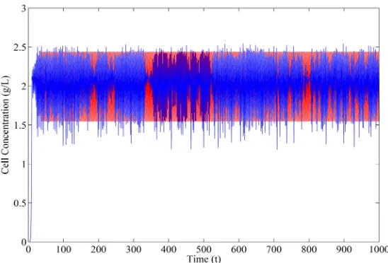
 . Furthermore, Xiao in [9] introduced the High strong order

[image:10.595.239.508.222.418.2]

stochastic Runge-Kutta methods for stochastic differential equations in case of Stratonovich with scalar noise. Since our model is in Stratonovich sense. Figure 1 and Figure 2 show the stability of Equation (3) and Equation (10) in positive equi-librium for cell growth of microorganism in fermentation process respectively.

Figure 1. Shows the stability of Equation (10). For deterministic part we use t0=0.00,

( )

0 0.0001

x = _, x_max=3.520_, µ_max=0.5_, σ=0.00, and b=0 and for stochastic part we chose same value just difference are σ =0.002, and b=1 respectively.

Figure 2. Illustrates the stability of Equation (10). For stochastic part we chose the 0 0.00

t = _, x

( )

0 =0.0001, xmax=3.520, µmax=1.99, b=1, and σ=0.021. For de-terministic part we use σ =0.00, b=0, t0=0.00, x

( )

0 =0.0001, xmax=3.520,

max 0.21

[image:10.595.241.507.474.663.2]

DOI: 10.4236/am.2019.108047 669 Applied Mathematics The blue line indicates the simple path of Equation (10) and the red line shows the simple path of Equation (3) respectively. In Figure 1 and Figure 2, the differ-ence are between the value of σ µ, max. The blue line indicates the simple path of Equation (10) and the red line shows the simple path of Equation (3) respective-ly. Figure 1 and Figure 2 are plotted under H1.

In both Figure 1 and Figure 2 lag phase is the luck of random fluctuations due to microbes are adopt with each other. Therefore, no growth takes place in this phase. Contrariwise, in stationary phase microbes fight with each other for food and space and the behavior of cell proliferation of microorganism is differ-ent in phases at fermdiffer-entation process. As time evolves, the system illustrates the intrinsic variability of the competing within species and deviations from expo-nential growth arise. It happens as a result of the nutrient level and toxin con-centration achieves a value which can no longer support the maximum growth rate. So, the stochastic fluctuations mainly affect the logistic growth of microor-ganism and for more see Remarks 3.1.

Remark 4.1: The red line shows the simple path of Equation (3) and the blue line indicates the simple path of Equation (10) respectively. If

σ

→ ±∞_{, there is}

no phases for cell growth which means this random fluctuations will destroy the phases in fermentation process on the other hands the process will tend to infinity. Remark 4.2: Figures 1-4 show the stability of Equation (3) and Equation (10) in different equilibrium points. Figure 3 and Figure 4 are plotted under H1 option 2. The thick red line illustrates the stability of Equation (10) without Ornstein-Uhlenbeck process. It is thick in stationary phase due to the growth rate µmax, is increased, compare the value of µmax with three others Figures.

5. Conclusion

[image:11.595.239.504.494.674.2]

This research is conducted on stability of stochastic logistic model with Ornstein-Uhlenbeck process for cell growth of microorganism in fermentation.

Figure 3. Shows the stability of Equation (10). For deterministic part we use t0=0.00,

( )

0 0.0001

[image:12.595.235.509.71.257.2]

DOI: 10.4236/am.2019.108047 670 Applied Mathematics

Figure 4. Illustrates the stability of Equation (10). For stochastic part we chose the 0 0.00

t = _, x

( )

0 =0.0001, xmax=2.09, µmax=2.2, µmax=0.21, b=1, and σ =0.02. For deterministic part we use σ=0.00, b=0, t0=0.00, x

( )

0 =0.0001, xmax=2.09,

max 2.2

µ = _.

This research proved that Equation (10) has a unique positive solution (see Theorem 3.1). Moreover, we proved that Equation (10) was stochastically stable in zero solution and positive equilibrium point (see Theorem 3.2 and Appendix A Theorem 1) and viewed in Figure 1 and Figure 2 and Appendix A. For nu-merical simulation we used SRK4 method to show the reality of this research. If the

σ

→ ±∞_{, the result will be infinity which means that there are no phases for}

cell growth. On the other hand, it will not preserve the stochastically stable. If 0 max max

x >x >µ _{, what will happen? Unfortunately, there are some impediments}

here which need some further investigation in future perspective.

Acknowledgements

This work is jointly supported by the National Natural Science Foundation of China under Grant Nos. 61573291, the Fundamental Research Funds for Central Universities XDJK2016B036.

Conflicts of Interest

The author declares no conflicts of interest regarding the publication of this pa-per.

References

[1] Ayoubi, T., Rosli, N., Bahar, A. and Salleh, M.M. (2015) Time Delay and Noise Ex-plaining the Behaviour of the Cell Growth in Fermentation Process. AIP Confe-rence Proceedings, 1643, 547-554. https://doi.org/10.1063/1.4907493

[2] Bahar, A. and Mao, X. (2004) Stochastic Delay Population Dynamics. International Journal of Pure and Applied Mathematics, 11, 377-400.

DOI: 10.4236/am.2019.108047 671 Applied Mathematics Clostridium acetobutylicum. Master Thesis, Universiti Malaysia Pahang, Pahang. [4] Burrage, K. and Burrage, P.M. (1996) High Strong Order Explicit Runge-Kutta

Me-thods for Stochastic Ordinary Differential Equations. Applied Numerical Mathe-matics, 22, 81-101. https://doi.org/10.1016/S0168-9274(96)00027-X

[5] Burrage, P.M. (1999) Runge-Kutta Methods for Stochastic Differential Equations. Ph.D. Thesis, University of Queensland, Queensland, Australia.

[6] Ariffin, N.N.A., Rosli, N. and Kasim, A.M. (2017) Stability Analysis of 4-Stage Sto-chastic Runge-Kutta Method (SRK4) and Specific StoSto-chastic Runge-Kutta Method (SRKS1.5) for Stochastic Differential Equations.In: Kor, L.K., Ahmad, A.R., Idrus, Z. and Mansor, K., Eds., Proceedings of the 3rd International Conference on Com-puting, Mathematics and Statistics, Springer, Singapore, 187-194.

https://doi.org/10.1007/978-981-13-7279-7_23

[7] Napoli, A. (2012) On a Class of Stochastic Runge Kutta Methods. International Journal Contemputation and Mathematics Sciences, 36, 1757-1769.

[8] Rüemelin, W. (1982) Numerical Treatment of Stochastic Differential Equations. SIAM Journal on Numerical Analysis, 19, 604-613. https://doi.org/10.1137/0719041

[9] Xiao, A. and Tang, X. (2016) High Strong Order Stochastic Runge-Kutta Methods for Stratonovich Stochastic Differential Equations with Scalar Noise. Numerical Algorithms, 72, 259-296. https://doi.org/10.1007/s11075-015-0044-0

[10] Evans, L.C. (2012) An Introduction to Stochastic Differential Equations. American Mathematical Society, Providence, RI. https://doi.org/10.1090/mbk/082

[11] Mazo, R.M. (2002) Brownian Motion: Fluctuations, Dynamics, and Applications. Oxford University Press, Oxford.

[12] Mishura, I.S. and Mishura, Y. (2008) Stochastic Calculus for Fractional Brownian Motion and Related Processes. Springer Science and Business Media, Berlin‎, Hei-delberg. https://doi.org/10.1007/978-3-540-75873-0

[13] Madihah, M.S., Ariff, A.B., Khalil, M.S., Suraini, A.A. and Karim, M.I.A. (2001) Anaerobic Fermentation of Gelatinized Sago Starch-Derived Sugars to Ace-tone—1-Butanol—Ethanol Solvent by Clostridium acetobutylicum. Folia Microbi-ologica, 46, 197-204. https://doi.org/10.1007/BF02818533

[14] Madihah, M.S. (2002) Direct Fermentation of Gelatinised Sago Starch to Solvent (Actone, Butanol and Ethanol) by Clostridium acetobutylicum. Ph.D. Thesis, Un-iversiti Putra Malaysia, ‎Serdang, Selangor, Malaysia.

[15] Bazli, M.K. (2010) Stochastic Modelling of the Clostridium acetobutylicum and Solvent Productions in Fermentation. Master Thesis, Universiti Technology Malay-sia, Malaysia.

[16] Aruğaslan, D. and Güzel, L. (2015) Stability of the Logistic Population Model with Generalized Piecewise Constant Delays. Advances in Difference Equations, 1, 173.

https://doi.org/10.1186/s13662-015-0521-8

[17] Jiang, D., Shi, N. and Li, X. (2008) Global Stability and Stochastic Permanence of a Non-Autonomous Logistic Equation with Random Perturbation. Journal of Ma-thematical Analysis and Applications, 340, 588-597.

https://doi.org/10.1016/j.jmaa.2007.08.014

[18] Liu, M. and Bai, C. (2015) A Remark on a Stochastic Logistic Model with Lévy Jumps. Applied Mathematics and Computation, 251, 521-526.

https://doi.org/10.1016/j.amc.2014.11.094

DOI: 10.4236/am.2019.108047 672 Applied Mathematics Applications, 433, 95-120. https://doi.org/10.1016/j.jmaa.2015.07.030

[20] Liu, Q., Jiang, D., Hayat, T. and Alsaedi, A. (2018) Long-Time Behavior of a Sto-chastic Logistic Equation with Distributed Delay and Nonlinear Perturbation. Physic A:Statistical Mechanics and Its Applications, 508, 289-304.

https://doi.org/10.1016/j.physa.2018.05.054

[21] Liu, M. and Wang, K. (2013) A Note on Stability of Stochastic Logistic Equation. Applied Mathematics Letters, 26, 601-606. https://doi.org/10.1016/j.aml.2012.12.015

[22] Mateos-Núñez, D. and Cortés, J. (2013) Stability of Stochastic Differential Equa-tions with Additive Persistent Noise. 2013 American Control Conference, Wash-ington DC, 17-19 June 2013, 5427-5432. https://doi.org/10.1109/ACC.2013.6580686

[23] Murray, J.D. (2001) Mathematical Biology II. Spatial Models and Biomedical Ap-plications. In: Interdisciplinary Applied Mathematics, Springer-Verlag, New York, 1-6.

[24] May, R.M. (2001) Stability and Complexity in Model Ecosystems. Princeton Uni-versity Press, Princeton, NJ.

[25] Arnold, L. (1972) Stochastic Differential Equations: Theory and Applications. Wi-ley, ‎Hoboken, NJ.

[26] Friedman, A. (1976) Stochastic Differential Equations and Their Applications. Academic Press, Cambridge, MA.

[27] Allen, E. (2007) Modeling with Itô Stochastic Differential Equations. Springer Science and Business Media,‎Berlin, Heidelberg.

[28] Khasminskii, R. (2011) Stochastic Stability of Differential Equations. Springer Science and Business Media,‎Berlin‎, Heidelberg.

[29] Mao, X. (1991) Stability of Stochastic Differential Equations with Respect to Semi-Martingales. Longman,‎Harlow.

[30] Mao, X. (1994) Exponential Stability of Stochastic Differential Equations. Marcel Dekker, New York.

[31] Mao, X. (2007) Stochastic Differential Equations and Applications. Elsevier, Ams-terdam, Netherlands.

[32] Gardiner, C.W. (2004) Handbook of Stochastic Methods for Physics, Chemistry and the Natural Sciences (Springer Series in Synergetics). Springer, Berlin‎, Heidelberg. [33] Rosli, N., Bahar, A., Su Hoe, Y. and Abd Rahman, H. (2010) Stochastic Model of

DOI: 10.4236/am.2019.108047 673 Applied Mathematics

Appendix A

Theorem 1: Equation (10) under the following assumption is globally asymp-totically stable in zero solution a.s (almost surely).

(H2): For 0≤t0,µmax < <0 x0< <σ xmax, then the limt→∞x t

( )

=0. Proof: An application of Itô’s formula for Equation (10) ([27], p. 95) leads to

( )

(

)

( )

( ) ( )

( )

( )

( )

( )

( )

( ) ( )

( )

( )

( )

( )

2 2 2

max

max

2

2 2 2

max 2

max

d ln

1 _{1 d d d}

1 _{1 d d}

2

A

B x t

x t

x t t x t bW t t x t W t

x t x

x t

x t t x t bW t dt x t W t

x x t

µ σ σ

µ σ σ

    =   −  − +            − +   −  − +          (32)

Equation (32) has two parts A and B. So,

( ) ( )

2

( )

( )

2 2

( )

( )

max

max

1 x t d d d

A x t t x t bW t t x t W t

x

µ   σ σ

= _ − _ − +

 

and

( ) ( )

( )

( )

( )

( )

2

2 2 2

max

max

1 x t d d d .

B x t t x t bW t t x t W t

x

µ σ σ

   

=  −  − + 

   

 

To simplify the B we have

( )

_{( )}

_{( )}

_{( )}

_{( )}

2

2 2 max

max

1 x t d d d

B t x t bW t t x t W t

x

µ σ σ

    =  −  − +       

( )

( )

( )

( )

( )

( )

(

)

( )

( )

( )

( )

(

)

2 max max max max 2 2 2 2 2

1 d 2 1 d

d d

d d

x t x t

B t t

x x

x t bW t t x t W t

x t bW t t x t W t

µ µ σ σ σ σ         =_  −  _ + _  −  _         × − + + − +

( )

( )

( )

(

( )

( )

( )

( )

)

( )

( )

( )

( )

(

)

(

( )

( )

)

( )

( )

(

)

(

( )

( )

)

(

( )

( )

)

2

2 max 2

max max max 2 2 max max max 2 2 2 2

2 2 2

d d 2 d d d

2 d d d d

d d d

2 d d d

x t

B t t x t t t t

x x

t x t t x t bW t t x t W t

x

x t bW t t x t W t x t bW t t

x t bW t t x t W t x t W t

µ µ

µ

µ σ σ

σ σ σ

σ σ σ

 _{ }    =_ × − _{× + }  _       + _ − _× − +   + − + + − + − +

Using these facts dt dt× =0,d dt w t×

( )

=0 and dW t

( )

×dW t

( )

=dt ([32], p. 87) and somewhat lengthy calculation we have

( )

4 4 _{d .}

B=σ x t t

DOI: 10.4236/am.2019.108047 674 Applied Mathematics

( )

(

)

_{( )}

( ) ( )

( )

( )

( )

( )

( )

(

( )

)

2 max max

2 2 4 4

2

1

d ln 1 d d

1

d d

2

x t

x t x t t x t bW t t

x t x

x t W t x t t

x t µ σ σ σ    =   −  −      − + _+  (33)

( )

(

)

( )

( )

( )

( )

( )

(

( )

)

max max

2 4 2

d ln 1 d d

1

d d

2

x t

x t t x t bW t t

x

x t W t x t t

µ σ σ σ    =  −  −      + _−  (34)

( )

max 01 _max( ) d 0 ( ) ( )d 20 ( ) ( )d 1₂ 40 2( )d

e

t x s _{s b x s W s s}t t_{x s W s} t_{x s s}

x

x t µ σ σ σ

  − − + −       ∫ ∫ ∫ ∫

= (35)

where W t

( )

is Brownian motion and taking expectation from both sides of above equation. We know the expectation of Brownian motion is zero ([10], Sec-tion 3.2.3, p. 43), we get

( )

max

( )

4 2

( )

max

0 0 0

max

exp d d d

2

t t t

E x t E x s s x s s s

x

µ σ _µ

  

= − − +

    

  _{ }

 



∫

∫

∫

 (36)

Takes limit

( )

max

( )

4 2

( )

max

0 0 0

max

lim lim exp d d d

2

t t t

t E x t t E x x s s x s s s

µ σ _µ

→∞ →∞    = − − +        _{ }  



∫

∫

∫

(37)

( )

max 0

( )

4 0 2

( )

0

max max

d d d

lim lim exp

2

t t t

t t

x s s x s s s

E x t E

x t t t

µ σ _µ

→∞ →∞       = − − +     _{  }     

∫

∫

∫

₍₃₈₎

For 0≤ ≤t T and based on ([10], p. 66 and p. 69) the 2

( )

0 d

T

x s s< ∞

∫

and

( )

0 d

T

x s s< ∞

∫

. Therefore

0 max d

lim e .

t _s t t t E µ           →∞ ∫           (39)

Under H2 yields

0 max d

lim e 0.

t _s t _t t E µ           →∞ ∫     =       (40)

Therefore, Equation (38) becomes

( )

lim 0.

t→∞x t =

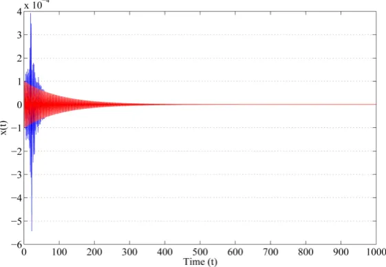
Ultimately, our claim is proved.  For plotting Figure 5 we use t0=0.00, x

( )

0 =0.0001, xmax =3.5250,

max 0.0091

[image:17.595.255.492.74.226.2]

DOI: 10.4236/am.2019.108047 675 Applied Mathematics

Figure 5. Shows the stability of Equation (10) with different value of parameters.

Figure 6. Illustrates the stability of Equation (10) with different value of parameters.

[image:17.595.234.515.263.457.2]