Statistical Approach to Mitigating 3G Interference to GPS in 3G Handset

Int. J. Communications, Network and System Sciences, 2010, 3, 730-736

doi:10.4236/ijcns.2010.39097 Published Online September 2010 (http://www.SciRP.org/journal/ijcns)

Statistical Approach to Mitigating 3G Interference to GPS

in 3G Handset

Taher AlSharabati, Yinchao Chen

University of South Carolina Columbia, South Carolina, USA E-mail: [email protected], [email protected] Received June 10, 2010; revised July 18, 2010; accepted August 22, 2010

Abstract

In this paper, we show how statistical decision theory can be used to solve real life product problems. Global Positioning System (GPS) performance in a mobile handset degrades whenever it is simultaneously used with a 3G data or voice service. This degradation is due to the 3G transmitter interference. Mitigation meth-ods to interference in GPS have been proposed. However, most of these methmeth-ods depend on hardware and signal processing or just hardware solutions. In some cases, it maybe difficult to implement these hardware meth-ods, especially in mobile handsets due to its small size, printed circuit board (PCB) layout issues and the added cost. In this paper, a novel signal processing statistical algorithm approach isproposed to mitigate the 3G interference to GPS. This statistical approach utilizes the knowledge of the statistical characteristics and distributions of both the GPS signal and noise. Then the method utilizes the probabilities to make a sta-tistical decision to remove the effect of noise. This method does not require room on the PCB of the mobile handset and therefore no layout challenges arise. In addition, cost is minimized and the product turn in cycle is shortened. This paper offers theoretical as well as practical insight to the GPS operation during 3G call inside the mobile phone.

Keywords:Detection and Estimation, Global Positioning System (GPS), Satellite Acquisition, Wide Band

Code Division Multiple Access (WCDMA)

1. Introduction

Global Positioning System (GPS) plays a major role in our daily lives. Its applications extend from naval, aero-space, first time emergency responders and location based-finding and directions in cell phones to name a few.

The existence of GPS in cell phones presents its own challenges since it co-exists with other services such as 3G WCDMA and GSM carriers [1].

The spatial distance or proximity of these services and subsystems and their components inside the cell phone is very small. Especially since the mobile handset is being packed with as many services as possible with the smallest form factor. This distance is small enough to the point where it does not present enough attenuation to the 3G transmitted Radio Frequency (RF) signals toward other receivers inside the handset. This, in turn, will present itself as interference to the receivers of the services that exist in the handset especially the GPS receiver. The effect of the distance on the attenuation or path loss of the transmitted signal strength is governed by the equation:

2 32.4 10log( )

A  rf (1)

where A is the attenuation in dB, f is the frequency of the transmitted signal and r is the distance between the transmitter antenna and the GPS receiver.

T. ALSHARABATI ET AL. 731

1710 MHz and that of WCDMA band IV is 1712.4 MHz. The frequency separation is less than 135 MHz.

It should be mentioned that architecture and system engineers do a thorough interference lineup analysis and calculations to assess the effects of different scenarios of the effects of interference of each band to itself and others with the given components of the subsystems before or on the onset of any transceiver chipset deployment. The effects of interference, if not mitigated, on receivers and the GPS receiver in particular are severe. These effects could range from degradation in user position accuracy or loss of satellite acquisition. This situation, when it happens to a receiver in a product like mobile phones, is called “de sense” i.e. the receiver is “de sensed”. In [1], the GPS receiver was de sensed by 5.5 dB. Shown in Figure 1 is a bar graph of the GPS satellites where eight of them have been acquired based on an acquisition metric of 2.5, where the horizontal axis is the satellite number and the vertical axis is the metric value, (Permission from [3]) when there is no 3G interference added to the data collected in [3]. Any satellite with an acquisition metric of 2.5 and above is considered acquired.

2. Analysis

In the following we present an analysis and examples for calculating two of the important parameters of the GPS receiver, namely; the average signal strength and the root mean squared (RMS) code tracking error.

2.1. Calculating the Average Signal Strength

The average carrier strength (Cav) (orCs) of the ac-quired satellites can be calculated based on Equation (9) in [4]. Equation (9) is repeated here for clarity purposes for the case1Dband assuming that 20.0332 (_2 _{is the normalized GPS code tracking error variance}

in units of sec2 _{[5], D is the two sided GPS correlator}

spacing and

r c

b T (2)

b is the normalized bandwidth, assumingr6MHz,Tc is the chip period ):

From this equation, the carrier to noise power ratio

s o

C N is:

dB 21.67 s

o C

dB

N 

.

Assuming system noise figure (NF) of 2dB and ther-mal noise power (No) of -174dB/Hz. From:

o s o

C N NF C N

av    (3)

av

C ~ = –150 dBm. This is the average signal strength or

carrier power of one of the acquired satellites. Figure 2 shows a plot of the average carrier power of the acquired satellites of Figure 1. The horizontal axis is the satellite number, while the vertical axis is the average carrier signal strength in dBm. Note how the values correspond to the metric values in Figure 1.

2.2. Calculating the RMS Code Error

One of GPS measurement accuracy parameters is the root mean squared (RMS) code tracking error in units of meters. Let’s denote the RMS code tracking error as

then [5],

*c 

  (4) where σ is the standard deviation in units of chips [6] and c is the speed of light. Each chip period is approxi-mately1s. For example, for the above case where

2 _0.0332

  ,  54.66 m. This is the code tracking error. Figure 3 displays the RMS code tracking error (in meters) of the acquired satellites. It is evident from this plot and that of Figure 2 how the average signal power affects this parameter. The stronger the power is; the less the error is and therefore the accurate the user position is.

3. Procedure

3.1. GPS Data and 3G Noise Generation

Being inside the phone, the GPS receiver suffers the most interference from the 3G transmitters inside the User Equipment (UE) while they are transmitting. From this point on, the 3G transmitted signals will be referred to as 3G noise because they present themselves as noise to the GPS receiver. The GPS data used in this paper are data collected in [3], which is data output of the ADC in that platform. The 3G noise will be simulated on the ba-seband level by using the WCDMA Quadrature Phase Shift Keying (QPSK) modulation scheme which is:

2 2

(1 0.5 ) 1 1 2

( ) ( ) 1 , 1 Db (9) in [4]

1

2 (2 )

L L

s s

o o

B B T b

D

T_c C b b C

T D

N N

 _



 

 

  _{  }

 _   _   

  

  _

 

T. ALSHARABATI ET AL. 732

2 3 4 5 6 7 8 9 10 11 12 13 14 15 16 17 18 19 20 21 22 23 24 25 26 27 0 1 2 3 4 5 6 7 8 9 10 11 12 13 14 15

Acq uisition Results

Acq uired Satellite's Nu m b er

Acq u is it io n M e tr ic

Not acqu ired sign als Acq uired sig nals

Figure 1. Number of acquired satellites when 3G noise is not present.

3 4 5 6 7 8 9 10 11 12 13 14 15 16 17 18 19 20 21 22 23 24 25 26 -151 -150.5 -150 -149.5 -149 -148.5 -148 -147.5 -147 -146.5 -146 -145.5 -145

Averag e Carrier P ow er of Ac q uired S atellites

Acq uired Satellites' Nu m b ers

A v er age C a rr ie r P o w e r C a v e ( d B m )

Figure 2. Plot of the average power of the acquired satel-lites.

3 4 5 6 7 8 9 10 11 12 13 14 15 16 17 18 19 20 21 22 23 24 25 26 20 25 30 35 40 45 50 55 60 65

RM S Cod e Tracking Error of Acqu ired S atellites

Acq uired Satellites' Nu m b ers

C o d e T ra c k in g E rro r E (m )

Figure 3. Plot of RMS code tracking error of the acquired satellites.

3 ( ) ( ( ) cos( ₄) ( )sin( ₄)) 2

( ), ( ) 1

I Q

G IF IF

I Q

Vrms

V t d t w t d t w t

d t d t

 

   

 

(5) where d tI( ), ( ) d tQ are the in phase and quadrature phase

baseband components of the data streams (which are random and normally distributed with zero mean and variance of one) and wIF is the intermediate frequency of the down converted signal. The 3G noise is sampled at the rate of the sampling frequency of the ADC in [3]. Then the 3G and GPS data are added together to form the GPS plus interference signal.

3.2. Determining 3G Noise Level

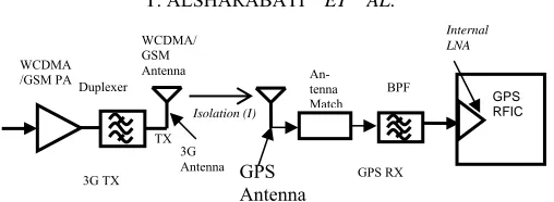
This task will take into consideration the total system architecture components of both the 3G transmit (3G TX) section and GPS receive section. Figure 4 shows a block diagram of a typical GPS-3G coexistence scenario [1]. The GPS section could be the hardware platform in [3]. Going from right to left; the heart of the GPS (GPS RX) receiver is the GPS Radio Frequency Integrated Chip (RFIC). Most of GPS RFICs have on board cross func-tional sections that span from RF to baseband. The SiGe 4120L [8] is one of SiGe’s GPS line of products. It has a low noise amplifier (LNA) on board and it outputs serial IQ data. So, its functionality span from RF to bits. A bandpass filter is used to filter out any signal outside the designed bandwidth of the GPS RX. At the forefront is the GPS antenna and antenna matching circuitry to bring the antenna impedance to a 50-ohm system. On the in-terfering 3G TX side, the TX-RX 3G antenna accom-modates both the WCDMA and GSM carrier bands. Then, the WCDMA/GSM Power Amplifier (PA) along with the duplexer.

Based on typical values of 3GPP WCDMA transmitter noise into GPS, values of 3G noise into GPS [9] (–140 dBm/Hz), duplexer insertion loss and spatial isolation, a value of Vrms (3G noise) in Equation (5) was calculated. This value came to be ~0.28 mV. In these calculations (for illustration purposes only), the spatial isolation is assumed to be 15 dB, the total receive line up gain is ~100 dB in 50 ohm system. First the power (PdB) of the

interferer was calculated and then it was converted to voltage based on a 50 ohm system:

dB noise into GPS + Lineup GaindB +

IsolationdB = 55 dB P 

 (6)

30 dBw

p  pdB (7)

2 10 log( / 50)

dBw rms

P   V (8)

0.28

rms

V mV

733

Figure 4. Typical co-existence 3G-GPS scenario.

4. Approach to the Algorithm

Previous published work has focused on suggesting either a combination of signal processing and hardware or just hardware solutions to mitigating the interference. In [7], antenna null steering was suggested to minimize Wide Band (WB) RF interference (RFI). While this me-thod works in products other than cell phones, it is diffi-cult to implement in the cell phone because it requires complex implementation of antenna design, RF front end electronics, feedback and signal processing. This method can not be implemented in the cell phone due to its com-plexity and immaturity for mobile phone environment. Other methods are proposed to prevent pulsed RFI [7]. While the methods just mentioned aimed at preventing interference from occurring, they do not mitigate the effects of interference after it happens. These methods do not offset the effects of errors generated once the interfer-ence is mixed along the line up and down converted to baseband with the desired GPS signal. Instead, a statisti-cal method is proposed to mitigate these errors.

The GPS data output from the ADC is Gaussian dis-tributed with zero mean and therefore their probability distribution function is normal and is in the form of:

2 2 1 ( ) 2 x

p x e 

 



 (9)

Figure 5 shows that distribution and weights in bar graph of the values and therefore it gives the probability of each value output from the Analog to Digital Con-verter (ADC). The red trace is the Normal distribution fit of the data. The horizontal axis are the values output from the ADC, the vertical axis are their weights. This figure does not literally give the probability values, but it shows the weights of these values.

5. Algorithm and Results

5.1. Mitigation Algorithm Development

The receiver tries to make a decision or best guess about a symbol si given that r was received. In other words, the

receiver tries to decide the probability of s given that r was received; p(s|r) based on the test statistic:

( | ) ( )i i

T  p r s p s (10)

Since the data follow the Gaussian distribution, then for N = 2 [10], where N is the number of dimensions of the signal space:

2 2 ( ) 2 ( | ) 2 i r s i e p r s



 

 

 (11)

and (10) becomes;

2 2 ( ) 2 ( | ) ( ) ( ) 2 i r s

i i i

e

p r s p s p s



 

 

 (12)

( )i

p s is the probability of the noise free quantized output GPS signal from the ADC and  is the standard deviation of the 3G noise. The novelty of this approach is as follows: since the Coarse Acquisition (C/A) code of the satellites is comprised of 1’s and –1’s (–1 for 0), the prototype messages can be reduced to two levels, namely; 1 and –1 and therefore calculating the probabilities in Figure 5 reduces to calculating the probabilities of the negative values of the signal and the probabilities of the positive values of the signal. We just need to recover the right phase of the signal. The decision reduces down to deciding whether a 1 or a –1 is being sent. In this case (12) generates two values:

2 2

( ) 2

(1| ) ( ) ( 0)

2

i

r s

i i i

e

p s p s p s



 

 

  (13)

and

2 2

( ) 2

( 1 | ) ( ) ( 0)

2

i r s

i i i

e

p s p s p s



 

 

   (14)

The decision goes to the one with the higher statistic.

5.2. Results

To determine user position, the GPS receiver has to ac-quire at least four satellites. Figure 6 shows the results of acquisition of GPS data plus 3G noise when no detection algorithm is used [2], namely PRN#: 15, 18, 21. From the results, only three satellites were acquired, not enough to determine user position. While after using the detection algorithm, five satellites (Figure 7) are ac-quired, namely PRN#: 6, 15, 18, 21, and 22. This will

WCDMA/ GSM Antenna Internal LNA GPS RFIC Isolation (I) TX BPF WCDMA

/GSM PA_Duplexer An-tenna Match 3G

Antenna

3G TX GPS GPS RX

T. ALSHARABATI ET AL. 734

help the GPS receiver in calculating the user position even if the user is using the mobile handset in either a data call or a voice call.

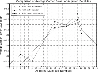
Based on Equations (2), (3) and (10) in [4], values of the average carrier power (Cav) were approximated and a comparison plot for three cases was obtained. The first case corresponds to the acquired satellites in Figure 1 where the results are for the raw data where no 3G noise was added to the data and therefore no detection algo-rithm was used. The second case corresponds to the

ac-quired satellites in Figure 6 where 3G noise was added to the data and no detection and estimation algorithm was used. The third case corresponds to the acquired satellites in Figure 7 where 3G noise was added to the data and the detection and estimation algorithm was used. Figure 8 shows such a comparison. It is evident from this plot how the proposed detection algorithm and estimation not only recovers the satellites lost due to noise, but it improves the average detected power of those satellites.

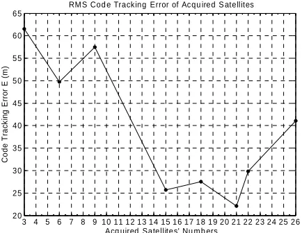
By using (4), a comparison was made for the code

-0.5 - 0.4 - 0.3 -0.2 -0.1 0 0.1 0.2 0.3 0.4

0 5 10 15 20 25 30

Dis cre tiz ed G P S Data O u tpu t of ADC

De

n

s

it

y

Pro ba bility D en sity D is trib ution o f G PS D ata

GPS data GPS Data F it

Figure 5. Distribution of GPS data from the ADC in [3].

Figure 6. Results of acquisition when no detection used. GPS data GPS data Fit

0 1 2 3 4 5 6 7 8 9 10 11 12 13 14 15 16 17 18 19 20 21 22 23 24 25 26 27 28 29 30 31 32 33 0

0.5 1 1.5 2 2.5 3 3.5 4 4.5 5

Ac qu isition re sults

Sa tellite nu mber

Ac

qu

is

it

ion

M

e

tr

ic

T. ALSHARABATI ET AL. 735

0 1 2 3 4 5 6 7 8 9 10 11 12 13 14 15 16 17 18 19 20 21 22 23 24 25 26 27 28 29 30 31 32 33

0 1 2 3 4 5 6 7 8

Acq uisition Results wtih N ew Detection Alg orithm

Satellites' n um ber

A

c

q

u

is

it

io

n

M

e

tr

ic

Not acquired signals A cquired signals

Figure 7. Results of acquisition when using detection algorithm.

3 4 5 6 7 8 9 10 11 12 13 14 15 16 17 18 19 20 21 22 23 24 25 26

-151 -150.5 -150 -149.5 -149 -148.5 -148 -147.5 -147 -146.5 -146 -145.5 -145

Com p arison of Average C arrier Power of Acqu ired S atellites

Acq uired Satellites' Nu m b ers

A

v

e

ra

g

e

Ca

rr

ie

r P

o

w

e

r Ca

v

e

(

d

B

m

)

3G Noise Added-No D etec tion

No 3G Noise-No D etection

3G Noise Added-Detection Used

Figure 8. Comparison of average carrier power of acquired satellites when (1) No 3G noise added. (2) 3G noise added-no de-tection algorithm used. (3) 3G noise added- dede-tection algorithm used.

3G Noise Added-No Detection No 3G Noise-No Detection

T. ALSHARABATI ET AL. 736

3 4 5 6 7 8 9 10 11 12 13 14 15 16 17 18 19 20 21 22 23 24 25 26 20

25 30 35 40 45 50 55 60 65

C o mp ariso n of R M S C od e Tra ck ing E rro r o f A cq uired S atellites

Ac qu ire d S atellite s' Nu mb ers

C

o

d

e

T

ra

c

ki

n

g

E

rro

r E

(m

)

3G Noise Added-No D etec tion No 3G Noise-No D etection 3G Noise Added-Detection Used

Figure 9. Comparison of RMS code tracking error of acquired satellites when (1) No 3G noise added. (2) 3G noise added-no detection algorithm used. (3) 3G noise added- detection algorithm used.

tracking error for the same three cases as shown in Fig-ure 9. The standard deviation was calculated for each tracked satellite. It is seen how the proposed algorithm reduces the error by showing less numbers in meters. This means that the user position is more accurate for the satellites acquired with noise and detection used than under noise without detection algorithm. It should be mentioned that the situation in Figure 6 is very optimistic. In many cases, the GPS receiver loses track of all satel-lites and hence no GPS fix can be obtained. The sug-gested algorithm guarantees to recover most if not all the satellites that are tracked as if the 3G noise is not present.

6. Conclusions

A cross functional effort has been displayed in this paper. The effort spanned from presenting architectural analysis and calculations for a 3G-GPS RF TX-RX system fo-cusing on the interference related aspects and sources, to estimating the average power of the received signal, to laying out the algorithm analysis and derivation of the mitigation scheme. We showed how the mitigation scheme can recover the acquisition of the satellites that were lost due to the interference. Also, the average car-rier power and RMS code tracking error of the recovered satellites are improved and therefore the user position accuracy is improved even though the mobile handset is in a 3G data or voice service when using the GPS service. This algorithm could be implemented at the phasing stage of a mobile handset development and manufacturing.

7. References

[1] T. Sharabati and Y. Chen, “Mitigating 3G Carrier Inter- ference to GPS Due to Co-Existence in 3G Handset,” IEEE NAECON, 2009, pp. 86-91.

[2] T. Sharabati, “Proposal for Mitigating 3G Interferrence to GPS,”University of South Carolina, South Carolina, 2009. [3] K. Borre, D. M. Akos, N. Bertelsen, P. Rinder and S. H.

Jensen, “A Software Defined GPS and Galileo Receiver Birkhauser,” Birkhauser, Boston,2007.

[4] W. B. John and R. K. Kevin, “Extended Theory of Early-Late Code Tracking for A Band limited GPS Receiver,” Navigation, Journal of the Institute of Navigation, Vol. 47, No. 3, 2000, pp. 211-226.

[5] W. B. John, “Effect of Narrowband Interference on GPS Code Tracking Accuracy,” ION NTM, 26-28 January 2000, pp. 16-27.

[6] B. Michael and A. J. V. Dierendonck, “GPS Receiver Architecture and Measurements,” Proceedins of the IEEE, Vol. 87, No. 1, 1999, pp. 48-64.

[7] P. Ward, “Interference Heads Up,” GPS World, Vol. 19, No. 6,June 2008, pp. 64-73.

[8] S. Semiconductor, “SE4120L GNSS Receiver IC,” June 2008.

[9] A. Technologies, “UTMS1700/2100(1710-1755MHz) and UMTS1700 (1750-1785MHz),” Avago Technologies,AV02- 1907EN, 2009.

[10]W. Couch Leon II, “Digital and Analog Communication Systems,” 3rd edition, Collier Macmillan, New York, 1990.