Randomized low rank Dynamic Mode Decomposition for motion detection

Randomized Low-Rank Dynamic Mode Decomposition for Motion

Detection

N.Benjamin Erichson, Carl Donovan

PII:

S1077-3142(16)00050-3

DOI:

10.1016/j.cviu.2016.02.005

Reference:

YCVIU 2385

To appear in:

Computer Vision and Image Understanding

Received date:

25 July 2015

Revised date:

11 December 2015

Accepted date:

6 February 2016

Please cite this article as: N.Benjamin Erichson, Carl Donovan, Randomized Low-Rank Dynamic

Mode Decomposition for Motion Detection,

Computer Vision and Image Understanding

(2016), doi:

10.1016/j.cviu.2016.02.005

ACCEPTED MANUSCRIPT

Highlights

• Fast and robust decomposition of a matrix representing a spatial grid through time.

• Rapid approximation for robust principal component analysis.

• Competitive performance in terms of recall and precision for motion detection.

ACCEPTED MANUSCRIPT

Randomized Low-Rank Dynamic Mode Decomposition for

Motion Detection

N. Benjamin Erichsona,∗_{, Carl Donovan}a

a_{School of Mathematics and Statistics, Univ. of St Andrews, UK}

Abstract

This paper introduces a fast algorithm for randomized computation of a low-rank

Dy-namic Mode Decomposition (DMD) of a matrix. Here we consider this matrix to

repre-sent the development of a spatial grid through time e.g. data from a static video source.

DMD was originally introduced in the fluid mechanics community, but is also suitable for

motion detection in video streams and its use for background subtraction has received

little previous investigation. In this study we present a comprehensive evaluation of

back-ground subtraction, using the randomized DMD and compare the results with leading

robust principal component analysis algorithms. The results are convincing and show

the random DMD is an efficient and powerful approach for background modeling,

allow-ing processallow-ing of high resolution videos in real-time. Supplementary materials include

implementations of the algorithms inPython.

Keywords: dynamic mode decomposition; robust principal component analysis; randomized singular value decomposition; motion detection;

background subtraction; video surveillance;

1. Introduction

The demand for video processing is rapidly increasing, driven by greater numbers of

sensors with greater resolution, new types of sensors, new collection methods and an ever

wider range of applications. For example, video surveillance, vehicle automation or

wild-life monitoring, with data gathered in visual/infra-red spectra or SONAR, from multiple

∗_{Corresponding author}

Email address: [email protected](N. Benjamin Erichson)

ACCEPTED MANUSCRIPT

sensors being fixed or vehicle/drone-mounted etc. The overall result is an explosion in

the quantity of high dimensional sensor data. Motion detection is often the fundamental

building block for more complex video processing and computer vision applications, e.g.

object tracking or human behavior analysis. In practice, there are many different types

of sensors giving data suitable for object extraction, however we focus here on video data

provided by static optical cameras, noting the findings generalize to other data types.

In this case, the change in position of an object relative to its surrounding environment

can be detected by intensity changes over time in a sequence of video frames. The

chal-lenge therefore is to separate intensity changes corresponding to moving objects from

those generated by background noise i.e. dynamic and complex backgrounds. From a

statistical point of view this can be formulated as a density estimation problem, aiming

to find a suitable model describing the background. Moving objects can then be

identi-fied by differences from the reconstructed background from the video frames, via some

thresholding, as illustrated in Figure 1. In practice, the problem of finding a suitable

video frame

background model

foreground mask threshold

(•)

d video

stream

τ

Figure 1: Illustration of background subtraction

model is difficult and often ill-posed due to the many challenges arising in real videos,

e.g., dynamic backgrounds, camouflage effects, camera jitter or noisy images, to name

only a few. One framework for tackling these challenges is provided by subspace

learn-ing techniques. Recently, robust principal component analysis (RPCA) has been very

successful in separating video frames into background and foreground components [1].

However, RPCA comes with relatively high computational costs and it is of limited

util-ity for real-time analysis of high resolution video. Hence, in light of increasing sensor

resolutions there is a need for algorithms to be more rapid, perhaps by approximating

ACCEPTED MANUSCRIPT

A competitive alternative is Dynamic Mode Decomposition (DMD) — a data-driven

method allowing decomposition of a matrix representing both time and space [2]. Due

to the unique properties of videos (equally spaced time with high temporal correlation),

DMD is well suited for motion detection, as first demonstrated by Grosek and Kutz [3].

1.1. Related work

Bouwmans [4] or Sobral and Vacavant [5] provide recent and comprehensive reviews

of methods for background modeling and related challenges. Among the many different

techniques, the class of (robust) subspace models are prominent. PCA can be considered

a traditional technique for describing the probability distribution of a static background.

However, PCA has some essential shortcomings and many enhancements have been

pro-posed since the method was first propro-posed for background subtraction by Oliver et al.

[6], e.g. adaptive, incremental or independent PCA. A review of those traditional

sub-space models and related issues is provided by Bouwman [7]. While DMD is related to

PCA and shares some of the same limitations, it can overcome others to greatly improve

the performance. Grosek and Kutz [3] have shown that DMD can be seen in fact as an

approximation to robust PCA (see also [8]). The idea of RPCA is to separate a matrix

Ainto a low-rank Land sparse componentS

A=L+S (1)

This can be formulated as a convex optimization problem that minimizes a combination

of the l2 and l1 norm. Applied to video data, the low-rank component describes the

relatively static background environment, which is allowed to gradually change over time,

while the second component captures the moving objects. This approach has gathered

substantive attention for foreground detection since the idea was first introduced by

Cand`es [9] - further extended by Zhou [10] for also capturing entry-wise noise. Bouwmans

and Zahzah [1] recently provided a comparative evaluation of the most prominent RPCA

implementations, whose results show LSADM [11] and TFOCS [12] algorithms perform

best in extracting moving objects in terms of the F-measure. Guyon et al. [13] show in

detail how the former algorithm can be used for moving object detection.

The problem formulation via RPCA leads to iterative algorithms with high

ACCEPTED MANUSCRIPT

Decomposition (SVD), so clearly the algorithms may be accelerated by using faster

ap-proximate SVD, aiming to find only the k dominant singular values. Liu et al. [14]

present a Krylov subspace-based algorithm for computing the firstksingular values with

high precision. They showed that their LMSVD algorithm can reduce the computational

time of RPCA substantially. Later they showed even greater computational savings with

their Gauss–Newton method based SVD algorithm [15]. If high precision is not the main

concern then approximate Monte-Carlo based SVD algorithms can be interesting

alter-natives [16, 17]. A different approach is via randomized matrix algorithms, which are

surprisingly robust and provide significant speed-ups, while being simple to implement

[18]. Halko et al. [19] and Gu [20] provide comprehensive surveys of randomized

algo-rithms for constructing approximate matrix decompositions, while Mahoney [21] gives

a more general overview. One successful approximate robust PCA algorithm using a

randomized matrix algorithms is given in GoDec [22].

1.2. Motivation and contributions

A core building block of the DMD algorithm, as for RPCA, is the SVD. As noted,

traditional deterministic SVD algorithms are expensive to compute and with increasing

data they often pose a computational bottleneck. We propose the use of a fast,

prob-abilistic SVD algorithm, exploiting the rapidly decaying singular values of video data.

Randomized SVD is a lean and easy to implement technique for computing a robust

approximate low-rank SVD [19]. Compared to deterministic truncated or partial SVD

algorithms, we gain computational savings in the order of 10 to 30 times. The next effect

is to increase speed of about 2 to 3 times with randomized DMD, rather than

determin-istic SVD based DMD. Hence, randomized DMD may facilitate real-time processing of

videos. Moreover, randomized SVD and DMD are embarrassingly parallel and we show

that the computational performance can benefit from a Graphics Processing Unit (GPU)

implementation. To demonstrate the applicability for motion detection, we have

eval-uated and compared dynamic mode decomposition on a comprehensive set of synthetic

and real videos with other leading algorithms in the field.

The rest of this paper is organized as follows. Section2 presents randomized SVD as

an approximation to the deterministic algorithms. Section 3 first introduces DMD and

ACCEPTED MANUSCRIPT

background modeling. Finally a detailed evaluation of DMD is presented in section 4.

Concluding remarks and further research directions are given in section5.

2. Singular Value Decomposition (SVD)

Matrix factorizations are fundamental tools for many practical applications in signal

processing, statistical computing and machine learning. SVD is one such technique, used

for data analysis, dimensionality reduction or data compression. Given an arbitrary real

matrixA_∈Rm×n _{we seek a decomposition, such that}

A=UΣV∗ (2)

where U∈Rm×m_{and V∈R}n×n _{are orthogonal matrices, andΣ∈R}m×n _{is a diagonal}

matrix with the same dimensions asA[23]. The columns ofUandVare both

orthonor-mal, called right and left singular vectors respectively. The singular values denoted as

σi are the diagonal elements of Σ sorted in decreasing order. While we assume a real

matrix here, for generality we use the Hermitian transpose denoted as∗_.

In practice we may be interested in a low-rank approximation ofAwith target rank

k m, n. Choosing the optimal target rank k is highly dependent on the task, i.e. whether one is interested in a very good reconstruction of the original data or in a very

low dimensional representation of the data. The reconstruction error for a low-rank

approximation:

kA₋UkΣkVk∗kF =σk+1 (3) is given by the singular valueσk+1, where the indexFdenotes the Frobenius norm. Thus,

a reasonable small singular value gives a low reconstruction error, and we can denote k

in this case as the effective rank of the matrix A. It can be proven that the exact low

rank approximation is provided by the deterministic SVD, however the computational

costs can be tremendous for large-scale problems, in particular for unstructured data. In

the following, we present a faster randomized algorithm [19].

2.1. A Randomized SVD Algorithm

Randomized matrix algorithms are approximate algorithms for linear algebra

ACCEPTED MANUSCRIPT

an input matrix A _∈Rm×n _{and a desired target rank k}

m, n the randomized algo-rithm for computing the approximate low-rank SVD can be roughly divided into two

stages.

The first stage is concerned with finding a random low-dimensional subspace that

best captures the column space of A. Here the idea of random projections is used to

build the basis for the column space. We simply drawkrandom Gaussian vectorsxiand

compute the following random sketch

yi =Axi fori=1,2,....,k (4)

As a result from probability theory, it follows that the random vectors, and hence the set

{yi} are linearly independent. We can compute (4) more compactly as matrix-matrix

product

Y=AΩ (5)

whereΩ_∈Rn×k_{is a random Gaussian matrix. We then compute the QR-Decomposition}

ofY to obtain the orthonromal matrixQ_∈Rm×k _{so that}

A≈QQ∗A (6)

is satisfied.

In the second stage we project the input matrixAonto the low-dimensional subspace

B=Q∗A (7)

The action of the column space ofAis now restricted to the relatively small (ifkm, n) matrixB_∈Rk×n_{. Subsequently we can cheaply compute the deterministic SVD ofBas}

B=UΣV˜ ∗ (8)

The randomized algorithm can be justified as follows

A _≈ QQ∗_A

≈ QB

≈ Q ˜UΣV∗

≈ UΣV∗

ACCEPTED MANUSCRIPT

Thus we can recover the right singular vectors by computing

U_≈Q ˜U (10)

Algorithm (1) shows a prototype for computing the randomized SVD.1

Algorithm 1 Randomized SVD (rSVD)

Input: A∈Rm×n _{and target rankk.}

Require: m_≥n, intk_≥1 andkn.

1: procedurersvd(A,k)

2: Ω_←rand(n, k) .Drawn_×k random matrix.

3: Y_←A_∗Ω .Compute random sketch.

4: Q_←qr(Y) . Economic QR-decomposition.

5: B_←Q∗_{∗A .Projection.}

6: U˜, s,V←svd(B) .Deterministic SVD.

7: U←Q∗U˜ .Recover right singular vectors.

return U∈Rm×k_{, s∈R}k_,V∈Rn×k 8: end procedure

Remark 1. Common choices for generating the random matrix Ω are the normal or

uniform distribution.

The computational time can further reduced by first computing the QR-decomposition

ofBand then computing the SVD of the even smaller matrixR∈Rk×k _{(see Voronin et}

al. [24] for further details).

The approximation error of a randomized SVD can be decreased by introducing a

small oversampling parameter p. This means, instead of drawing k random vectors,

we generate k+p samples, so that the likelihood of spanning the correct subspace is

increased. A small oversampling parameterp(e.g. p= 5) is generally sufficient. Further,

computingqpower iterations can increase the accuracy:

Y= (AA∗)qAΩ (11)

1_{See supplementary materials for a more detailed algorithm andPythonimplementation with}

over-sampling parameter and subspace iterations.

ACCEPTED MANUSCRIPT

The power iterations drive the spectrum ofYdown and the approximation error, which

is proportional to the spectrum, decays exponentially with the number of iterations.

Even if the signal-to-noise ratio is low, q = 1,2 power iterations already achieve good

results. For numerical reasons a practical implementation should use subspace iterations

instead of power iterations [20]. Halko et al. [19] showed that the approximation error

of randomized SVD has the following error bound [19], if the oversampling parameter is

chosen equal tok, i.e. l:= 2k

EkA₋UlΣlVl∗k

=σl+1

"

1 + 4

r

2min(m, n) l₋1

# 1 2q+1

(12)

2.2. Computational Costs

SVD is often the bottleneck in practical large-scale applications. Many different

meth-ods for computing the SVD have been proposed and optimized for different problems,

exploiting certain matrix properties. Thus, giving a detailed overview of the

computa-tional costs is difficult.

In short however, the time complexity for the ordinary deterministic SVD algorithms

is O(mn2_{) ifm > n, while modern partial SVD methods based on rank-revealing}

QR-factorization can reduce the time complexity to O(mnk) [25]. The randomized SVD

algorithm using random sampling, as we have presented it here, needs two passes over

the input matrix and also has asymptotic costs ofO(mnk). Hence, theoretically we have

the same costs asymptotically - however from a practical point of view, it is much cheaper

to compute a matrix-matrix multiplication than a column-pivoted QR factorization. The

costs can be further deceased by exploiting certain matrix properties to compute a fast

matrix-matrix multiplication of (5) to O(mnlog(k)) floating point operations. For

ex-ample, the Subsampled Random Fourier Transform (SRFT) as proposed by Woolfe et

al. [26] can be used.

In practice, the computational time of (randomized) SVD algorithms is also heavily

driven by the computational platform used, the specific implementation and whether the

matrix fits into the fast memory. An advantage of randomized SVD is that it can benefit

from parallel computing. For example, permitting a GPU implementation, leading to

dramatic acceleration [24]. This is because the GPU architecture enables fast generation

ACCEPTED MANUSCRIPT

3. Dynamic Mode Decomposition (DMD)

DMD is a data-driven method, fusing PCA with time-series analysis (Fourier

trans-form in time) [2]. This integrated approach for decomposing a data matrix overcomes the

PCA short-coming of performing an orthogonalization in space only. DMD is an

emer-gent technique in the fluid mechanics community for analyzing the dynamics of non linear

systems and was originally proposed by Schmidt [27] and Rowley et al. [28]. Allowing the

assessment of spatio-temporally coherent structures, with almost no underlying

assump-tions makes DMD interesting for video processing. Specifically, the resulting low-rank

features are of interest for modeling the background of surveillance videos. In addition,

DMD also allows predictions to be made about short-time future states of video streams

[29].

To compute the DMD, an ordered and evenly spaced data sequence describing a

dynamical system is required. This applies naturally to videos, where a data matrix

D _{∈ R}m×n _{can be constructed so that the columns are n consecutive grey coloured}

videos frames f _∈Rm_{. The elements d}

jt ofD refer to the intensity of a pixel in space

(j) and time (t). As is common in the DMD literature, we denote such a data matrix

also as snapshot sequence. Further, it is reasonable to assume that two consecutive video

frames are related to each other in time. Mathematically, we can establish the following

important relationship

ft+1=Mft (13)

stating that there exists an unknown underlying linear operator M ∈Rm×m _that

con-nects two consecutive video frames [27]. Here the indext ∈ {1,2, ..., n} is denoting a frame in time. It turns out that M is the Koopman operator whose eigenvalue decom-position describes the evolution of a video sequence [30]. Hence, the goal of DMD is to

find an approximate decomposition ofM2_{. It is also interesting to note that, while the}

operator Mis considered to be linear, its eigenvectors and eigenvalues can also describe

nonlinear dynamical systems.

2_{Traditionally, the problem of obtaining the operator Mwas formulated in terms of a companion}

matrix in order to emphasize the deeper theoretical relationship to the Arnodli Algorithm and the

Koopman operator. We refer to [27,28] for further theoretical details.

ACCEPTED MANUSCRIPT

3.1. Low-Rank Dynamic Mode Decomposition Algorithm

To compute the DMD we proceed by first arranging the data matrixD_∈Rm×n _into

two matrices:

X=h f1 | f2 | ft | ... | fn−1

i

∈Rm×(n−1) ₍₁₄₎

Y=h f2 | f3 | ft+1 | ... | fn i

∈Rm×(n−1) ₍₁₅₎ The left snapshot sequence X is approximately linked to the right sequence Y by the

operator Mas follows

Y_≈MX (16)

This is in fact a well known linear least squares problem

minkY−MXk2

F (17)

An estimate can be computed using the pseudo-inverse [31] as follows

M=YX†=YVΣ−1U∗ (18)

where U _{∈ R}m×n _{and V}

∈ Rn×n _{are denoting the left and right singular values}

re-spectively, and Σ_∈Rn×m _{the diagonal matrix with the corresponding singular values.}

However, this direct approach of computing the operatorMmight not be feasible when

dealing with high dimensional data, like videos. Instead it is more desirable to reduce

the dimension first using a similarity transformation in order to find an approximate

operator M˜ ∈Rn×n _as

˜

M=U∗MU (19)

In fact it can be shown thatMandM˜ have the same eigenvalues [25]. Using the similarity

transformation draws a connection between DMD and PCA by projecting M onto the

principal components (left singular vectors)U. We obtainM˜ by plugging (18) into (19)

as follows (note thatUis a matrix with orthonormal columns and henceU∗U=I)

˜

M=U∗MU=U∗YVΣ−1 (20)

It can be seen that the SVD plays a central role in computing the DMD. Computing the

ACCEPTED MANUSCRIPT

of video data (with rankkn) allows us to use fast approximate low-rank decomposi-tion techniques, e.g., randomized SVD (rSVD) as described in Secdecomposi-tion2. We denote this

approach using rSVD for computing an approximate low-rank dynamic mode

decompo-sition with a specified target rank k, as randomized DMD (rDMD). In this case, the

dimension of the linear operator reduces to M˜ _∈Rk×k_{. The structure of M˜ is revealed}

by computing the eigenvalue decomposition of M˜ as

˜

MW=ΛW (21)

whereW_∈Ck×k _{is the eigenvector matrix andΛ}

∈Ck×k_{is a diagonal matrix containing}

the eigenvalues λ. The dynamic modesΦ _∈Cm×k _{are then computed by relating the}

eigenvectors back toMas either [27]

Φ= [φ1, ..., φk] =UW (22)

or more generally as [30]

Φ=YVΣ−1W (23)

We favor the latter approach.

The original data matrix D can be reconstructed by noting that the snapshots can

be represented as the linear combination [32]

ft≈ k X

i=1

biφiλti−1 (24)

where λi denotes theith eigenvalue,φi theith dynamic mode andbi the corresponding

amplitude. Since bi is time independentf1 reduces to

f1≈

k X

i=1

biφi=Φb (25)

The parameter vector b_∈Ck _{can be estimated by the linear least squares method [3].}

Figure 2illustrates how the approximate low-rank DMD can be expressed as

D≈ΦBVand (26)

ACCEPTED MANUSCRIPT

where B_∈Ck×k _{is a diagonal matrix of the amplitudes}

B=         b1 bi . .. bk         (27)

andVand∈Ck×n is the Vandermonde matrix of the eigenvalues

Vand=        

1 λ1 · · · λn1−1 1 λ2 · · · λn2−1 ..

. ... . .. ...

1 λk · · · λn_k−1         (28)

From the Vandermonde matrix it is clear that temporal dynamics, retrieved by the DMD,

consists of single (distinct) frequencies.

≈

Space Time Dynamic modes Amplitudes Temporal evolu on Time Space Video frames

Figure 2: Illustration of low-rank dynamic mode decomposition.

The prototype Algorithm (2) summarizes the method for computing the DMD using

rSVD.

3.2. DMD for Background Modeling

In the previous section we have seen how DMD can be used to decompose and

re-construct a matrix. However, using (26) for modeling the video background directly is

a bad strategy. Of course, we can hope that when computing the low-rank dynamic

mode decomposition, that the dominant dynamic modes are not corrupted by any

ACCEPTED MANUSCRIPT

Algorithm 2 Randomized DMD (rDMD)

Input: D_∈Rm×n _{and target rankk.}

Require: m≥n, integerk≥1 andkn

1: procedurerDMD(D,k)

2: X,Y←D . Left/right snapshot sequence.

3: U,s,V←rsvd(X, k) . Low-rank rSVD.

4: S←diag(s−1) . Diagonal matrix.

5: M←U∗∗Y∗V∗S . Least squares fit.

6: W, l_←eig(M) . Eigenvalue decomposition.

7: F_←Y_∗V_∗S_∗W . Compute modesΦ.

8: b_←lstsq(F,x1) . Compute amplitudes.

9: V_←vander(l) . Vandermonde matrix.

10: return F∈Cm×k_,b∈Ck_,V∈Ck×n 11: end procedure

train DMD on a set of clean video frames. However, that is an unrealistic scenario in

real world applications. More desirable is a decomposition into low-rank L(background

components) and sparse componentsS(foreground components) similar to RPCA [9]

D=L+S (29)

Unlike robust PCA, DMD is not capable of directly separating a matrix into these two

components. Instead, DMD allows us to compute an approximation to it. First let us

connect the DMD eigenvalues λto the Fourier modesω as follows [3]

ωi=

ln(λi)

∆t (30)

For standard videos we simply assume the time step ∆t = 1 and hence ωi = ln(λi).

By construction, the eigenvalues are complex. Hence the Fourier modes allow us to

reveal interesting properties about the relating dynamic modes. The real part of ω

determines the mode’s evolution over time, while the imaginary part is related to the

mode’s oscillations. Now let us rewrite (26) in terms of the Fourier modes for aklow-rank

ACCEPTED MANUSCRIPT

decomposition of a video matrix

D≈ΦBVand= k X

i=1

biφiexp(ωit) (31)

wheret= [0,1, ...,(n₋1)] is the time vector. From (31) it is clear that the Fourier modes dictate how the modes evolve, i.e., decay or grow in time. In light of this, the set of k

modes{φi}can be separated into a set that contains only Fourier modes{wl:kwlk 1}

who evolve slowly over time and corresponds to background modes. The second set{ws}

contains modes describing fast moving objects. Exploiting this, (31) can be rewritten as

D_≈X

i∈l

biφiexp(ωit) + X

i∈s

biφiexp(ωit) (32)

The background video can then be reconstructed as follows

L=X

i∈l

biφiexp(ωit) (33)

Foreground objects (sparse components) can be identified as difference between the

orig-inal video data and the background video L(discarding the imaginary part)

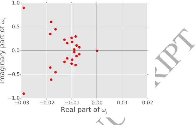
S=_kD₋L_k2 (34) We illustrate the concept on a real video in the following examples. Figure 3shows the

Fourier modes of a low-rank dynamic mode decomposition with target rankk= 25. The

Fourier mode_kω0k ≈0 identifies the background mode, shown in Figure4(b). However, using just the zero mode leads to a static background model. Figure 4 (c) shows that

the waving tree is captured as foreground object when using the zero mode only. Hence,

to better cope with dynamic backgrounds, it is favorable to select a subset of modes

kwbk 1 for background modeling. Using the first 3 modes decreases the false positive

rate, as shown in figure 4 (d). Deciding upon the number of modes used for modeling

the background was semi-arbitrary and we achieved qualitatively good results with 3 to

5 modes — whereas using the zero mode is computationally faster.

4. Experimental Evaluation

In this section we evaluate both the accuracy and computational performance of the

ACCEPTED MANUSCRIPT

−0.03 −0.02 −0.01

0.00

0.01

0.02

Real part of

ω

i

−1.0

−0.5

0.0

0.5

1.0

Im

ag

ina

ry

pa

rt

of

ω

i

Figure 3: Fourier modes corresponding to a low-rank dynamic mode decomposition.

(a) Original frame. (b) Zero mode.

(c) Foreground

reconstructed with zero

mode only.

(d) Foreground

reconstructed with the 3

[image:17.595.159.486.148.357.2]

smallest modes.

Figure 4: Illustration of background modeling using DMD.

ACCEPTED MANUSCRIPT

effectiveness of rDMD for detecting moving objects we use two benchmark datasets.

First, we test rDMD on ten synthetic videos from the BMC 2012 (Background Models

Challenge) dataset [33]. Further, to evaluate the performance on real videos, we use eight

videos from the ChangeDetection.net (CD) dataset [34]. The selected videos represent

challenging examples in motion detection. For example:

• Bootstrapping: A sequence of clean background images which are not available for training.

• Dynamic backgrounds: Moving objects which belong to the background like waving trees, rain or snowfall.

• Illumination changes: Gradual illumination changes of the environment due to fog or sun.

• Camouflage: Foreground objects which have the same pixel intensity as back-ground elements, i.e. same color.

4.1. Evaluation Measures

To evaluate the performance of background subtraction algorithms, a binary

fore-ground mask using a suitable distance measured(·) has to be computed

Xt(j) =   

1 ifd(fjt−bjt)> τ

0 otherwise (35)

For instance, the Euclidean distance is a common choice for measuring the distance

be-tween pixels of the actual video and the re-constructed background frame [35]. However,

more sophisticated measures can be formulated and allow adaptive thresholding. The

resulting vectorXtis called the foreground ormotion mask and its elements are binary

x∈ {0,1}. In the outcomes, 1 classifies a pixel belonging to a foreground object, oth-erwise 0 as a background element. Thus we can visualize the classification results as an

confusion matrix

Truth

0 1

Prediction 0 TN FN #pred neg

1 FP TP #pred pos

#true neg #true pos

ACCEPTED MANUSCRIPT

where TP denotes the (number of) True Positive predictions, i.e. pixels which are

cor-rectly classified as belonging to a moving foreground object. Similarly TN denotes the

(number of) True Negative predictions, i.e. pixels which are correctly classified as

back-ground. False Positive (FP) and False Negative (FN) are the respective misclassifications

for foreground and background elements. Based on the confusion matrix we can compute

the following evaluation measures.

Recall (also called sensitivity, true positive rate or hit rate) measures the algorithm’s

ability to correctly detect pixels belonging to foreground objects. It is computed as the

ratio of predicted true positives to the total number of true positive foreground pixels

Recall= TP

TP + FN (37)

Precision (also called false alarm rate or true positive accuracy) measures how

confi-dent we can be that a positive classified pixel actually belongs to a foreground object. It

is computed as the ratio of predicted true positives to the total number of pixels predicted

as foreground objects

Precision= TP

TP + FP (38)

Specificity (also called true negative rate) measures the algorithm’s ability to correctly

predict pixels belonging to the background. It is computed as the ratio of true negatives

to the total number of true negative foreground pixels

Specificity= TN

TN + FP (39)

The F-measure combines recall and precision as their harmonic mean, weighting both

measures evenly, defined as

F= 2_×Recall×Precision

Recall + Precision (40)

More general definitions of the F-measure also allow different weighting schemes.

From (35) it is obvious that the classification results depend on a pre-defined fixed

threshold τ. To get a global understanding of the algorithm’s behaviors the evaluation

measures can be computed over a range of different thresholds. The results can then

be visualized using precision-recall and Receiver Operator Characteristics (ROC) curves.

ACCEPTED MANUSCRIPT

changes in the class distribution [36]. In particular in dynamic environments such as

videos, the number of pixels belonging to foreground objects can vary significantly over

frames and is generally much less then the number of pixels belonging to the background.

A further advantage of using ROC curves is the convenient way to summarize the

per-formance with a global single scalar value measuring the Area Under the Curve (AUC).

The perfect ROC curve has an AUC of 1, while random guessing yields an AUC of 0.5.

Thus a method with an AUC close to 0.5 or below can be considered as useless, while a

method with a higher AUC is preferred.

4.2. Results

DMD is formulated as a batch algorithm here, i.e, previous modeled sequences do

not effect the following. This allows the algorithm to adapt to changes in the scene, e.g.,

illumination changes. Also, foreground objects that become background objects (like a

recently parked car) can be better captured. On the other hand, it does not allow for

dealing with ‘sleeping’ foreground objects. The performance varies with the number of

modes and the length of the snapshot sequence. Our results show that a snapshot length

of about 100 to 300 video frames can be separated with a very low number of modes,

e.g. k ∈ {9,11, ...,15}. If the video is less noisy, a lower number of dynamic modes is sufficient. However, depending on how fast the foreground objects are moving, using less

than 100 frames often leads to a poor detection performance. Another important issue is

the choice of the initial condition used for computing the amplitudes. The default option

is to use the first frame of the sequence, as stated in (25), however we often achieved

better results using the median frame instead. Another interesting option is to recompute

the amplitudes for small chunks of the sequence. This allows better capture of sudden

illumination changes.

For the rDMD algorithm, two further tuning parameters pand q can be specified.

The former is the oversampling parameter and the latter controls the number of power

iterations of the rSVD algorithm. For computing rDMD in the following we keep the two

parameters fixed asp= 2 andq= 1. This parameter setting recovers almost exactly the

results achieved with the ordinary DMD algorithm.

We first illustrate in Figure5the performance of rDMD compared to ordinary DMD,

ACCEPTED MANUSCRIPT

the AUC and the F-measure, rDMD and DMD can be seen as a reasonable

approxima-tion. The results also show that the performance difference between rDMD and DMD is

insignificant. As expected, DMD performs significantly better than PCA in terms of the

F-measure.

0.00 0.05 0.10 0.15 0.20

1-specificity 0.70 0.75 0.80 0.85 0.90 0.95 1.00 Re ca ll

DMD : AUC=0.952 rDMD : AUC=0.954 Robust PCA : AUC=0.969 PCA : AUC=0.952

0 20 40 60 80 100 120 140 Threshold 0.2 0.3 0.4 0.5 0.6 0.7 0.8 0.9 1.0 F-M ea su re DMD F=0.771 rDMD F=0.773 Robust PCA F=0.817 PCA F=0.658

(a) CD baseline video ’Highway’ frame 500 to 700.

0.00 0.05 0.10 0.15 0.20

1-specificity 0.70 0.75 0.80 0.85 0.90 0.95 1.00 Re ca ll

DMD : AUC=0.947 rDMD : AUC=0.945 Robust PCA : AUC=0.964 PCA : AUC=0.956

0 20 40 60 80 100 120 140 Threshold 0.2 0.3 0.4 0.5 0.6 0.7 0.8 0.9 1.0 F-M ea su re DMD F=0.828 rDMD F=0.827 Robust PCA F=0.832 PCA F=0.702

(b) CD baseline video ’Pedestrians’ frame 600 to 800.

Figure 5: Performance evaluation of rDMD, DMD, PCA and RPCA on two videos. The left column

presents ROC curves and the right column the F-measure. While RPCA performs best, DMD/rDMD

can be seen as a good approximation.

Table 1 shows the results of randomized DMD for the ten synthetic videos of the

BMC dataset and compares them with three leading robust PCA algorithms: LSADM,

TFOCS and GoDec. LSADM [11] is a principal component pursuit algorithm, while

TFOCS [12] is a quantization-based principal component pursuit algorithm. GoDec

[22] is an approximated RPCA algorithm based on bilateral random projections and

like rDMD uses the concept of randomized matrix algorithms. Overall the average

F-measure shows that the detection performance of rDMD is about 4% lower than the

ACCEPTED MANUSCRIPT

RPCA algorithms. The slightly poorer performance is due to the Street 512 and Rotary

522 videos, emulating windy scenes with additional noise. In these cases the background

is very dynamic and the precision of the DMD algorithm is decreased. However, this

problem can be compensated for by post-processing the obtained foreground mask with

a median filter. The overall performance of this approach leads to an improvement of

about 2%. The results on the other videos show that DMD is flexible enough to deal

with illumination changes like clouds, fog or sun.

Measure Street Rotary Average

112 212 312 412 512 122 222 322 422 522

LSADM

Goldfarb et al. [11]

Recall 0.874 0.857 0.906 0.862 0.840 0.878 0.880 0.892 0.782 0.830

-Precision 0.830 0.965 0.867 0.935 0.742 0.940 0.938 0.892 0.956 0.869

-F-Measure 0.851 0.908 0.886 0.897 0.788 0.908 0.908 0.892 0.860 0.849 0.880

TFOCS

Becker et al. [12]

Recall 0.910 0.843 0.867 0.903 0.834 0.898 0.892 0.892 0.831 0.877

-Precision 0.830 0.965 0.899 0.889 0.824 0.924 0.932 0.887 0.940 0.879

-F-Measure 0.868 0.900 0.882 0.896 0.829 0.911 0.912 0.889 0.882 0.878 0.885

GoDec

Zhou and Tao [22]

Recall 0.841 0.875 0.850 0.868 0.866 0.822 0.879 0.792 0.813 0.866

-Precision 0.965 0.942 0.968 0.948 0.902 0.900 0.921 0.953 0.750 0.837

-F-Measure 0.899 0.907 0.905 0.906 0.884 0.859 0.900 0.865 0.781 0.851 0.876

rDMD Recall 0.873 0.855 0.760 0.805 0.783 0.883 0.860 0.772 0.800 0.834 -Precision 0.887 0.912 0.902 0.900 0.656 0.896 0.907 0.876 0.902 0.770

-F-Measure 0.880 0.882 0.825 0.850 0.714 0.889 0.882 0.820 0.848 0.800 0.839

rDMD

(with median filter)

Recall 0.859 0.833 0.748 0.793 0.801 0.862 0.834 0.808 0.761 0.831

-Precision 0.906 0.935 0.924 0.916 0.879 0.922 0.936 0.892 0.941 0.894

-F-Measure 0.882 0.881 0.826 0.850 0.838 0.891 0.882 0.847 0.842 0.861 0.860

Table 1: Evaluation results of ten synthetic videos from the BMC dataset. For comparison, the results

of three other leading RPCA algorithms are presented, adapted from [1].

We show in Table2the evaluation results of 8 real videos from the CD dataset. The

videos are from three different categories: ‘Baseline’, ‘Dynamic Background’ and

‘Ther-mal’. At first glance the overall performance of the rDMD algorithm looks poor. This

can be related to several challenges faced here. While the performance on the two

base-line videos ’Highway’ and ’Pedestrians’ are good, issues arise for the other two basebase-line

videos. The PETS2006 is difficult, due to camouflage effects for the DMD algorithm, as

well as because some of the objects are sleeping foreground objects. The ‘Office’ shows

even more drastically that DMD cannot cope with sleeping foreground objects. However,

ACCEPTED MANUSCRIPT

overcome this problem. The two dynamic background videos show the same problem

as before with the synthetic videos. The recall rate is excellent, while the precision is

lacking. But again just using a simple median filter for pre-processing increases the

performance greatly. Figure 6shows some visual results for 3 selected videos. For

com-Figure 6: Visual results for 3 example frames from the CD Videos: Highway, Canoe and Park. The top

row shows the original gray scaled image and the second row the corresponding true foreground mask.

The third line shows the differencing between the reconstructed background and the original frame.

Rows four and five are the thresholded and median filtered foreground masks, respectively.

parison we show in Table 2 also the results of two algorithms leading the CD ranking.

The FTSG (Flux Tensor with Split Gaussian models) [37] algorithm is based on mixture

of Gaussians which won the 2014 CD challenge. The PAWCS (Pixel-based Adaptive

Word Consensus Segmenter) [38] is a word-based approach to background modeling.

While the raw results of DMD clearly cannot compete with the two mentioned highly

optimized methods, it can be seen that simple post-processing can accelerate the

perfor-mance substantially. Hence the object detection rate can be improved by learning from

other background modeling methods and using for example, a more elaborate threshold,

or integrating DMD into a system allowing background maintenance.

ACCEPTED MANUSCRIPT

Measure Baseline Dynamic Background Thermal Average

Highway Pedestrians PETS2006 Office Overpass Canoe Park Lakeside

PAWCS

St-Charles et al. [38]

Recall 0.952 0.961 0.945 0.905 0.961 0.947 0.899 0.520

-Precision 0.935 0.931 0.919 0.972 0.957 0.929 0.768 0.752

-F-Measure 0.944 0.946 0.932 0.937 0.959 0.938 0.829 0.615 0.887

FTSG

Wang et al. [39]

Recall 0.956 0.979 0.963 0.908 0.944 0.913 0.666 0.228

-Precision 0.934 0.890 0.883 0.961 0.941 0.985 0.724 0.960

-F-Measure 0.945 0.932 0.921 0.934 0.943 0.948 0.694 0.369 0.835

rDMD Recall 0.810 0.943 0.680 0.482 0.797 0.854 0.736 0.680

-Precision 0.789 0.756 0.703 0.560 0.194 0.201 0.610 0.448

-F-Measure 0.799 0.839 0.691 0.518 0.312 0.325 0.667 0.540 0.586

rDMD

(with median filter)

Recall 0.901 0.976 0.681 0.551 0.778 0.900 0.816 0.655

-Precision 0.899 0.945 0.713 0.642 0.929 0.937 0.744 0.571

-F-Measure 0.900 0.960 0.696 0.593 0.847 0.918 0.779 0.610 0.788

Table 2: Evaluation results of eight real videos from the CD dataset. For comparison, the results of

two algorithms from the CD ranking are presented.

4.3. Computational performance

We now evaluate the computational performance of rSVD and rDMD algorithm

re-spectively. Our implementations are written in Python3 _{using the multi-thread MKL}

(Intel Math Kernel Library) accelerated linear algebra library LAPACK. For the GPU implementation we are using NVIDIA CUDA in combination with the linear algebra libraries cuBLAS [40] andCULA [41]. To allow the comparison of rSVD with the fast LMSVD [14] algorithm we have used Matlab. All the computations were performed on a standard gaming notebook (Intel Core i7-5500U 2.4GHz, 8GB DDR3 L memory and

NVIDIA GeForce GTX 950M). It is important to note that in order to achieve any

com-putational advantage with rSVD the target rank has to bek < n

1.5, otherwise truncated

SVD would be faster. Another requirement is that the matrix fits into the fast memory.

4.3.1. Randomized SVD

Figure 7 shows the computational time for rSVD with LMSVD and a partial SVD

(svds) algorithm for two different sized matrices and a varying target rank. rSVD with

one subspace iteration can achieve time savings of about a factor 10 to 30. Comparing

to the LMSVD (with default options) the speed-up is about 5 to 8 times. However,

3_{Python Software Foundation. Python Language Reference, version 2.7. Available at}

ACCEPTED MANUSCRIPT

the reconstruction error shows that the LMSVD algorithm is more precise, in particular

when comparing to rSVD without subspace iterations.

0 20 40 60 80 100

Target rank

k 101 102 103 104 105

Tim

e i

n m

illi

se

co

nd

s

0 20 40 60 80 100

Target rank

k 0.0 0.2 0.4 0.6 0.8 1.0

Re

lat

ive

re

co

nst

ruc

tio

n e

rro

r

svds

lmsvd

rsvd

rsvd (q=1)

rsvd (q=2)

(a) Square (3000_×3000) random matrix.

0 20 40 60 80 100

Target rank

k 101 102 103 104 105

Tim

e i

n m

illi

se

co

nd

s

0 20 40 60 80 100

Target rank

k 0.0 0.2 0.4 0.6 0.8 1.0

Re

lat

ive

re

co

nst

ruc

tio

n e

rro

r

(b) Thin (1e5_×500) random matrix.

Figure 7: Computational performance of fast SVD algorithms on two random matrices for 5 different

target ranksk. Randomized SVD outperforms partial SVD (svds) and LMSVD, while LMSVD is more

accurate. Performing 1 or 2 subspace iterations improves the reconstruction error of rSVD

considerably. The time is plotted on a log scale.

4.3.2. Randomized DMD

For feasible real-time processing, our aim was to accelerate the ordinary DMD

algo-rithm by using a randomized matrix algoalgo-rithm for computing the SVD. Figure 8shows

the computational times we obtain with a randomized algorithm on videos with two

different resolutions. The randomized version allows us to accelerate the computational

ACCEPTED MANUSCRIPT

mentation. This allows processing of up to 180 frames per second for a 720x480 video.

For a 320x240 video it can increase the frames per second from about 300 up to 750. The

GPU accelerated DMD implementation benefits in particular from the fast computations

of dot products, QR-decomposition and the fast generation of random numbers. Using

a high-end graphic card can further improve the results, enabling real-time processing

of HD 720 videos and beyond. The limitation of a GPU implementation is that the

snapshot sequence has to fit into the graphic card’s memory.

320x240 720x480

Video resolution

0 100 200 300 400 500 600 700 800

Fra

me

s p

er

se

co

nd

(f

ps)

140 28 170 34 333 72 293 64 262 57 750 183

DMD

DMD (partial svd)

rDMD

rDMD (q=1)

rDMD (q=2)

GPU rDMD (q=2)

Figure 8: Comparison of the computational performance of DMD on real videos. Randomized DMD

(even with subspace iterations) outperforms DMD using a truncated or partial SVD algorithm. In

addition, using an GPU accelerated implementation can substantially increase the performance.

5. Conclusion

We have presented a fast algorithm for computing the low-rank DMD using a

ran-domized matrix algorithm. This subtle modification leads to substantial decreases in

computational time, enabling DMD to process videos with high resolutions in real-time.

Furthermore, the randomized version is of particular interest for parallel processing, e.g.

GPU accelerated implementations. Randomized matrix algorithms may be beneficial for

many other methods built on numerical linear algebra and in particular for those that

ACCEPTED MANUSCRIPT

The suitability of DMD for motion detection has been evaluated on synthetic and

real videos using statistical metrics. The results show that DMD can be seen as a

fast approximation of RPCA. The results compared to other robust PCA algorithms are

competitive, but the results of DMD compared to advanced statistical models leading the

CD ranking are less optimal in terms of accuracy metrics. However, we have also shown

that simple post-processing can enhance the results substantially. The performance can

be further improved by adaptive thresholds or by integration into a background modeling

system. This makes DMD interesting for applications where fast processing is more

important then extremely high precision.

In addition, we note that DMD is not a method purely designed for background

modeling. DMD comes with a rich mathematical framework, which offers potential for

interesting further research and applications beyond video. For example, interesting

research directions are opened by multi-resolution dynamic mode decomposition [42],

making the algorithm particularly interesting for the task of object tracking and motion

estimation. Another direction is compressed DMD for fast background modeling. Both

compressed and randomized DMD offer the opportunity to use importance sampling

strategies to model a more robust background.

Acknowledgment

For the many discussions and insightful remarks on dynamic mode decomposition

we would like to thank J. Nathan Kutz and Steven L. Brunton. We would also like to

express our gratitude to Leonid Sigal and the two anonymous reviewers for the many

helpful comments to improve this paper. N. Benjamin Erichson acknowledges support

from the UK Engineering and Physical Sciences Research Council (EPSRC).

References

[1] T. Bouwmans, E. H. Zahzah, Robust pca via principal component pursuit: A review for a

com-parative evaluation in video surveillance, Computer Vision and Image Understanding 122 (2014)

22–34. doi:10.1016/j.cviu.2013.11.009.

[2] J. N. Kutz, Data-Driven Modeling and Scientific Computation: Methods for Complex Systems and

Big Data, Oxford University Press, 2013.

ACCEPTED MANUSCRIPT

[3] J. Grosek, J. N. Kutz, Dynamic mode decomposition for real-time background/foreground

separa-tion in video (2014).arXiv:1404.7592.

[4] T. Bouwmans, Traditional and recent approaches in background modeling for foreground detection:

An overview, Computer Science Review 11-12 (2014) 31–66.doi:10.1016/j.cosrev.2014.04.001.

[5] A. Sobral, A. Vacavant, A comprehensive review of background subtraction algorithms evaluated

with synthetic and real videos, Computer Vision and Image Understanding 122 (2014) 4–21. doi:

10.1016/j.cviu.2013.12.005.

[6] N. Oliver, B. Rosario, A. Pentland, A bayesian computer vision system for modeling human

inter-actions, Pattern Analysis and Machine Intelligence, IEEE Transactions on 22 (8) (2000) 831–843.

doi:10.1109/34.868684.

[7] T. Bouwmans, Subspace learning for background modeling: A survey, Recent Patents on Computer

Science 2 (3) (2009) 223–234.

[8] T. Bouwmans, A. Sobral, S. Javed, S. K. Jung, E.-H. Zahzah, Decomposition into low-rank plus

additive matrices for background/foreground separation: A review for a comparative evaluation

with a large-scale dataset (2015). arXiv:1511.01245.

[9] E. J. Cand`es, X. Li, Y. Ma, J. Wright, Robust principal component analysis?, Journal of the ACM

58 (3) (2011) 1–37.doi:10.1145/1970392.1970395.

[10] Z. Zhou, X. Li, J. Wright, E. Candes, Y. Ma, Stable principal component pursuit, in: Information

Theory Proceedings (ISIT), 2010 IEEE International Symposium on, 2010, pp. 1518–1522. doi:

10.1109/ISIT.2010.5513535.

[11] D. Goldfarb, S. Ma, K. Scheinberg, Fast alternating linearization methods for minimizing the sum

of two convex functions, Mathematical Programming 141 (1-2) (2013) 349–382. doi:10.1007/

s10107-012-0530-2.

[12] S. Becker, E. J. Cand`es, M. C. Grant, Templates for convex cone problems with applications

to sparse signal recovery., Mathematical Programming Computation 3 (3) (2011) 165–218. doi:

10.1007/s12532-011-0029-5.

[13] C. Guyon, T. Bouwmans, E.-H. Zahzah, Moving object detection by robust pca solved via a

lin-earized symmetric alternating direction method, in: Advances in Visual Computing, Springer, 2012,

pp. 427–436.

[14] X. Liu, Z. Wen, Y. Zhang, Limited memory block krylov subspace optimization for computing

dominant singular value decompositions (2012).

[15] X. Liu, Z. Wen, Y. Zhang, An efficient gauss–newton algorithm for symmetric low-rank product

matrix approximations, SIAM Journal on Optimization 25 (3) (2015) 1571–1608. doi:10.1137/

140971464.

[16] A. Frieze, R. Kannan, S. Vempala, Fast monte-carlo algorithms for finding low-rank approximations,

Journal of the ACM 51 (6) (2004) 1025–1041.

[17] P. Drineas, R. Kannan, M. W. Mahoney, Fast monte carlo algorithms for matrices ii: Computing a

low-rank approximation to a matrix, SIAM Journal on Computing 36 (1) (2006) 158–183.

ma-ACCEPTED MANUSCRIPT

trices, Applied and Computational Harmonic Analysis 30 (1) (2011) 47–68. doi:10.1016/j.acha.

2010.02.003.

[19] N. Halko, P. G. Martinsson, J. A. Tropp, Finding structure with randomness: Probabilistic

algo-rithms for constructing approximate matrix decompositions, SIAM Review 53 (2) (2011) 217–288.

doi:10.1137/090771806.

[20] M. Gu, Subspace iteration randomization and singular value problems, SIAM Journal on Scientific

Computing 37 (3) (2015) A1139–A1173.doi:10.1137/130938700.

[21] M. W. Mahoney, Randomized algorithms for matrices and data, Foundations and Trends in Machine

Learning 3 (2) (2011) 123–224.doi:10.1561/2200000035.

[22] T. Zhou, D. Tao, Godec: Randomized low-rank & sparse matrix decomposition in noisy case, in:

International Conference on Machine Learning, ICML, 2011, pp. 1–8.

[23] D. S. Watkins, Fundamentals of Matrix Computations, 2nd Edition, John Wiley & Sons, Inc., New

York, NY, USA, 2002.

[24] S. Voronin, P.-G. Martinsson, Rsvdpack: Subroutines for computing partial singular value

de-compositions via randomized sampling on single core, multi core, and gpu architectures (2015).

arXiv:1502.05366.

[25] J. Demmel, Applied Numerical Linear Algebra, Society for Industrial and Applied Mathematics,

1997.doi:10.1137/1.9781611971446.

[26] F. Woolfe, E. Liberty, V. Rokhlin, M. Tygert, A fast randomized algorithm for the approximation

of matrices, Applied and Computational Harmonic Analysis 25 (3) (2008) 335–366.

[27] P. J. Schmid, Dynamic mode decomposition of numerical and experimental data, Journal of Fluid

Mechanics 656 (2010) 5–28.doi:10.1017/S0022112010001217.

[28] C. W. Rowley, I. Mezi`c, S. Bagheri, P. Schlatter, D. S. Hennigson, Spectral analysis of nonlinear

flows, Journal of Fluid Mechanics 641 (2009) 115–127.doi:10.1017/S0022112009992059.

[29] J. N. Kutz, X. Fu, S. L. Brunton, Multi-resolution dynamic mode decomposition (2015). arXiv:

1506.00564.

[30] J. H. Tu, C. W. Rowley, D. M. Luchtenburg, S. L. Brunton, J. N. Kutz, On dynamic mode

decomposition: Theory and applications (2013).arXiv:1312.0041.

[31] G. Golub, W. Kahan, Calculating the singular values and pseudo-inverse of a matrix, Journal of the

Society for Industrial & Applied Mathematics, Series B: Numerical Analysis 2 (2) (1965) 205–224.

[32] M. Jovanovic, P. Schmid, J. Nichols, Low-rank and sparse dynamic mode decomposition, Center

for Turbulence Research Annual Research Briefs (2012) 139–152.

[33] A. Vacavant, T. Chateau, A. Wilhelm, L. Lequievre, A benchmark dataset for outdoor

fore-ground/background extraction, in: Computer Vision–ACCV 2012 Workshops, Springer, 2013, pp.

291–300.

[34] Y. Wang, P.-M. Jodoin, F. Porikli, J. Konrad, Y. Benezeth, P. Ishwar, Cdnet 2014: an expanded

change detection benchmark dataset, in: IEEE Workshop on Computer Vision and Pattern

Recog-nition, IEEE, 2014, pp. 393–400.

[35] Y. Benezeth, P.-M. Jodoin, B. Emile, H. Laurent, C. Rosenberger, Comparative study of background

ACCEPTED MANUSCRIPT

subtraction algorithms, Journal of Electronic Imaging 19 (3) (2010) –.doi:10.1117/1.3456695.

[36] T. Fawcett, An introduction to roc analysis, Pattern Recogn. Lett. 27 (8) (2006) 861–874. doi:

10.1016/j.patrec.2005.10.010.

[37] R. Wang, F. Bunyak, G. Seetharaman, K. Palaniappan, Static and moving object detection using

flux tensor with split gaussian models, in: Computer Vision and Pattern Recognition Workshops

(CVPRW), 2014 IEEE Conference on, IEEE, 2014, pp. 420–424.

[38] P.-L. St-Charles, G.-A. Bilodeau, R. Bergevin, A self-adjusting approach to change detection based

on background word consensus, in: Applications of Computer Vision (WACV), 2015 IEEE Winter

Conference on, IEEE, 2015, pp. 990–997.

[39] R. Wang, F. Bunyak, G. Seetharaman, K. Palaniappan, Static and moving object detection using

flux tensor with split gaussian models, in: Computer Vision and Pattern Recognition Workshops

(CVPRW), 2014 IEEE Conference on, IEEE, 2014, pp. 420–424.

[40] J. Nickolls, I. Buck, M. Garland, K. Skadron, Scalable parallel programming with cuda, Queue 6 (2)

(2008) 40–53.doi:10.1145/1365490.1365500.

[41] J. R. Humphrey, D. K. Price, K. E. Spagnoli, A. L. Paolini, E. J. Kelmelis, Cula: hybrid gpu

accelerated linear algebra routines (2010).doi:10.1117/12.850538.

[42] J. N. Kutz, X. Fu, S. L. Brunton, Multi-resolution analysis of dynamical systems using dynamic

mode decomposition, in: Proceedings of the World Congress on Engineering, Vol. 1, WCE, 2015,