arXiv:1707.02989v1 [astro-ph.GA] 10 Jul 2017
THE SDSS-IV MANGA SAMPLE: DESIGN, OPTIMIZATION, AND USAGE CONSIDERATIONS
David A. Wake1,2,3, Kevin Bundy4,5, Aleksandar M. Diamond-Stanic6,2, Renbin Yan7, Michael R. Blanton8, Matthew A. Bershady2, Jos´e R. S´anchez-Gallego9, Niv Drory10, Amy Jones11, Guinevere Kauffmann11, David
R. Law12, Cheng Li13,14, Nicholas MacDonald9, Karen Masters15,16, Daniel Thomas15,16, Jeremy Tinker8, Anne-Marie Weijmans17, Joel R. Brownstein18
ABSTRACT
We describe the sample design for the SDSS-IV MaNGA survey and present the final properties of the main samples along with important considerations for using these samples for science. Our target selection criteria were developed while simultaneously optimizing the size distribution of the MaNGA integral field units (IFUs), the IFU allocation strategy, and the target density to produce a survey defined in terms of maximizing S/N, spatial resolution, and sample size. Our selection strategy makes use of redshift limits that only depend oni-band absolute magnitude (Mi), or, for a small subset of
our sample,Miand color (N U V −i). Such a strategy ensures that all galaxies span the same range in
angular size irrespective of luminosity and are therefore covered evenly by the adopted range of IFU sizes. We define three samples: the Primary and Secondary samples are selected to have a flat number density with respect to Mi and are targeted to have spectroscopic coverage to 1.5 and 2.5 effective
radii (Re), respectively. The Color-Enhanced supplement increases the number of galaxies in the
low-density regions of color-magnitude space by extending the redshift limits of the Primary sample in the appropriate color bins. The samples cover the stellar mass range 5×10⁸≤M
∗≤3×10¹¹M⊙/h2and
are sampled at median physical resolutions of 1.37 kpc and 2.5 kpc for the Primary and Secondary samples respectively. We provide weights that will statistically correct for our luminosity and color-dependent selection function and IFU allocation strategy, thus correcting the observed sample to a volume limited sample.
1. INTRODUCTION
The SDSS-IV MaNGA survey (Bundy et al. 2015; Blanton et al. 2017) is using the ARC 2.5m
tele-1
School of Physical Sciences, The Open University, Milton Keynes, MK7 6AA UK;[email protected]
2
Astronomy Department, University of Wisconsin-Madison, Madison, WI 53706, USA
3
Department of Physics, University of North Carolina Asheville, One University Heights, Asheville, NC 28804, USA
4
Dept. of Astronomy and Astrophysics, UC Santa Cruz, MS: UCO / LICK, 1156 High St, Santa Cruz, CA 95064, USA
5
Kavli IPMU (WPI), UTIAS, The University of Tokyo, Kashiwa, Chiba 277-8583, Japan
6
Department of Physics and Astronomy, Bates College, 44 Campus Avenue, Carnegie Science Hall, Lewiston, Maine 04240, USA
7
Department of Physics and Astronomy, University of Ken-tucky, 505 Rose St., Lexington, KY 40506-0057, USA
8
Center for Cosmology and Particle Physics, Department of Physics, New York University, 4 Washington Place, NY 10003, New York, USA
9
Department of Astronomy, Box 351580, University of Wash-ington, Seattle, WA 98195, USA
10
McDonald Observatory, University of Texas at Austin, 1 University Station, Austin, TX 78712-0259, USA
11
Max-Planck Institut fr Astrophysik, D-85741 Garching, Germany
12
Space Telescope Science Institute, 3700 San Martin Drive, Baltimore, MD 21218, USA
13
Department of Physics and Tsinghua Center for Astro-physics, Tsinghua University, Beijing 100084, China
14
Shanghai Astronomical Observatory, Nandan Road 80, Shanghai 200030, China
15
Institute of Cosmology and Gravitation, University of Portsmouth, Portsmouth, UK
16
SEPnet, South East Physics Network (www.sepnet.ac.uk)
17
School of Physics and Astronomy, University of St Andrews, North Haugh, St Andrews KY16 9SS, UK
18
Department of Physics and Astronomy, University of Utah, 115 S. 1400 E., Salt Lake City, UT 84112, USA
scope (Gunn et al. 2006) and the BOSS spectrographs (Smee et al. 2013) with its fibers bundled into multiple IFUs (Drory et al. 2015) to measure spatially resolved spectroscopy of ∼10,000 nearby galaxies. We have cho-sen to target a well defined sample that has uniform spa-tial coverage in units ofr-band effective radius along the major axis (Re), and an approximately flat stellar mass
distribution with 109 .M
∗/M⊙/h2 .1011. In this
pa-per, we discuss the motivation and methodology of the MaNGA sample selection, and we present the resulting sample in a way that allows for its use in statistical anal-ysis of galaxy properties.
The challenge of designing a survey like MaNGA is to balance the need for sample size, spatial coverage, and spatial resolution; these three parameters com-pete with each other for finite fiber resources. We have chosen a sweet spot in this multi-parameter space that best matches our science requirements (outlined in Bundy et al. 2015; Yan et al. 2016) in the context of a six-year survey duration, existing spectrographs, and telescope field of view. Since the sample design and the modifications to the BOSS spectrographs’ fiber feeds (Drory et al. 2015) occurred concurrently we were able to optimize both together to a considerable degree. Specifically, we determined the optimal IFU size com-plement within the confines of a total fiber budget and viable sample design. Fortuitously, the redshift range 0.02 . z . 0.1 that balances angular size versus reso-lution also delivers a target surface density that is well matched to the telescope field of view (3 degrees in di-ameter) and the roughly 1500 fibers with 2′′ diameters
hind-sight it is a lesson learned for planning future sur-veys. One of the aims of this paper is to demonstrate how, with adequate knowledge of target density, well-matched instrumentation can be optimally configured to achieve well-motivated survey science requirements.
A number of our design choices, such as an even sampling in stellar mass, roughly uniform radial cover-age, and a sample size in the thousands, are similar in spirit to those of the SAMI survey (Croom et al. 2012; Bryant et al. 2015). Such choices result naturally from a desire to efficiently study the local galaxy population and produce several similar features in the sample selec-tion approach, such as a stellar mass dependent redshift range. However, our ability to simultaneously design the IFU size distribution and sample selection using a tele-scope with a larger field does offer further advantages for optimization.
1.1. Design Strategy
A number of strategic and tactical choices inform tech-nical elements of the sample design. A starting point was to select from the well understood SDSS Main Sample (Strauss et al. 2002) with enhanced redshift complete-ness and remeasured photometry, as described in Section 2. Because the redshifts and global properties of SDSS galaxies are well known, the distributions of these prop-erties in the final MaNGA sample can be carefully con-structed by effectively weighting the MaNGA selection in order to maximize its scientific utility.
1. Sample size: Paramount is the requirement for a large, statistically powerful sample size, a choice that comes at the expense of higher quality data for individual galaxies within the sample. As de-scribed in Bundy et al. (2015), the specific argu-ment for sampling 10,000 galaxies arises from the desire to divide galaxies into 63 groups of ∼ 50 galaxies each. These groups, or bins (i) sample each of three “principal components” defining galaxy populations – stellar mass, SFR and environment; (ii) divide each “dimension” into 6 bins, sufficient to distinguish the functional form of trends across each dimension; and finally (iii) contain adequate counting statistics (galaxies) such that differences in mean properties between bins can be detected at the 5 sigma level even when the measurement pre-cision for individual galaxies is comparable to this difference. This optimization dovetails MaNGA’s scientific goals for statistical analyses of resolved galaxy samples, and complements existing, smaller data sets such as ATLAS3D (Cappellari et al. 2011), DiskMass (Bershady et al. 2010), and CAL-IFA (S´anchez et al. 2012), as well as forthcoming data from instruments such as MUSE (Bacon et al. 2010) and KCWI (Martin et al. 2010) capable of producing even higher fidelity data for more mod-est samples.
2. Sampling in stellar mass: We desire the MaNGA sample to have a roughly flat distribution in logM∗
so that studies of mass-dependent trends could make use of adequate numbers of high-mass galax-ies compared to more numerous low-mass systems. A flat stellar mass distribution requires an upper
redshift limit that is stellar mass dependent, so a larger volume is sampled for rarer high mass galax-ies.
3. Radial coverage: We desire roughly uniform radial coverage as defined by some multiple of the effective radius. This choice is motivated by the existence of well-known scaling relations that emphasize the importance of the relative length scale of galaxy stellar density profiles. Uniform spatial coverage in units of Re requires a lower redshift limit that
is stellar mass dependent, so larger more massive galaxies have the same angular size as smaller lower mass galaxies. MaNGA therefore samples the same relative extent of the declining surface brightness profile, but at the cost ofnotmaintaining the same physical spatial resolution across the sample.
4. Maximize spatial resolution and S/N: With cur-rent facilities, we wish to build a data-set of IFU spectroscopy for 10,000 galaxies with the maxi-mum possible per galaxy physical spatial resolu-tion, spectral coverage and resoluresolu-tion, and S/N per spatial element. These requirements lead to several inevitable tactical features of the selection criteria:
(a) to maximize the spatial resolution and total S/N requires the selection of galaxies at as low redshift as possible.
(b) to reach our goal of 10,000 galaxies requires a sufficiently broad redshift distribution so as to have enough galaxies per plate to maximize efficiency in IFU allocation.
1.1.1. Subsamples
The question of how to set the target radius motivated significant thought during the sample design. Smaller multiples of the effective radius would yield greater spa-tial resolution and more spaspa-tial samples with higher S/N. Larger radial coverage would contain more of the galaxy’s light, reach into the dark-matter dominated regime, and probe unchartered territory in the outskirts of galaxies. After studying a number of options, a compromise was reached to cover out to 1.5Re (the majority of the light
distribution) for two-thirds of the sample and to cover out to 2.5Refor one-third of the sample. Going to larger
radii, while compelling, was deemed too costly in terms of the number of spatial samples per IFU with very low S/N. The sample split was motivated by basic binning arguments (see Bundy et al. 2015) and officially adopted by the science team after the first year of observations.
With the main sample roughly flat in logM∗, it was
possible to consider a further optimization, that is bal-ancing the rest-frame color distribution (a proxy for star formation rate) at fixed M∗. In this way, rare
or undesirable, the supplemental sample could be eas-ily separated from the Primary sample, and in the worst case scenario, even ignored. With the risk mitigated, the decision was made to include the Color-Enhanced sup-plement in the selection.
To summarize, the final full MaNGA sample with which we began the survey consists of three main sub-samples. The Primary sample, which will initially make up 50% of the targets, is designed to be covered by our IFUs to 1.5Reand has a flat distribution in K-corrected
i-band absolute magnitude (Mi). The Secondary sample,
making up 33% of the initial targets, is again designed to have a flat distribution in Mi but with coverage to
2.5 Re. Finally, the Color-Enhanced supplement is
de-signed to add galaxies in regions of the N U V −i versus Mi color magnitude plane that are under-represented in
the Primary sample, such as high mass blue galaxies and low mass red galaxies, and will make up 17% of the ini-tial targets. The combination of the Primary and Color-Enhanced samples is called the Primary+ sample.
This complexity leads to the final strategic choice in the survey design:
5. Selection simplicity: While we have described the basic strategic and tactical motivations behind var-ious choices for the sample design, we were also driven to make the selection as simple and repro-ducible as possible. The implementation of the “weighting” described above to deliver a MaNGA sample with desired global distributions is carried out entirely through a set of selection criteria in-volving basic observables that are relatively model-independent: redshift, i-band luminosity, and, for the Color-Enhanced supplement, (NUV - i) color. Note that the selection does not depend on effec-tive radius explicitly (although a radius estimate is used when choosing what sized IFU to allocate to given galaxy target). We also emphasize that while much of the sample design studies made use ofM∗estimates, the final selection employsi-band
absolute magnitudes as a proxy for M∗.19 We did
not use M∗ estimates specifically in order to avoid
potential systematic biases and the use of a “black-box” estimator that may be difficult to reproduce.
1.2. Extant Instrumentation
Various aspects of the sample design are dependent on the nature of the MaNGA instrumentation. We highlight a few details here and refer to Drory et al. (2015) for more details.
The MaNGA instrumentation suite is composed of fiber-bundle IFUs dedicated to observing galaxy targets, with a number of additional IFUs and single fibers re-served for calibration. The total number of fibers, 1423, is limited by the size of the inherited BOSS spectro-graphs. The science IFUs contain circular, buffered op-tical fibers tightly arranged in a hexagonal format. This geometry enables IFUs of different sizes, with specific
19
For the initial IFU size distribution optimization process we used the stellar mass as estimated by the kcorrect code (Blanton & Roweis 2007) applied to the five band SDSS photom-etry. For the final samples we have switched to using just i-band absolute magnitude in order to simplify the selection function (see Section 4.1)
numbers of fibers for each IFU size. With a “live-core” fiber diameter of 2′′ and full outer diameter of 2′′.5, the
smallest science IFUs contains a central fiber and two outer, hexagonal rings for a total of 19 fibers and long-axis IFU diameter of 12′′.5. Other possible IFU sizes are 37 fibers (17′′.5), 61 fibers (22′′.5), 91 fibers (27′′.5), 127
fibers (32.′′5), 169 fibers (37′′.5), 217 fibers (42′′.5), and so
on. Choosing the largest IFU size as well as the optimal distribution of IFU sizes is a major focus of this paper.
Identical sets of the MaNGA instrumentation suite are installed in six SDSS “cartridges.” These sturdy, cylindrical structures house the light-collecting IFUs and fibers, the field-specific plug plate, and the out-put pseudo-slit, which is directed into the spectrographs when the cartridge is mounted on the telescope. The fer-rules and jacketing of single fibers and MaNGA IFUs are similar, with dimensions that facilitate hand-plugging of these elements into pre-drilled plates. As a result there is a “collision radius” that defines the minimum distance between plugged elements. For the MaNGA IFUs this distance is 120′′. The mounting of the plate in the
car-tridge makes use of a post that attaches to the center of the plate helping to deform the plate to the shape of the focal plane. This center post introduces a second “collision radius” about the center of the plate of 150′′.
The balance of this paper is organized as follows: In§2 we describe the construction of the parent catalogs from the NASA-Sloan Atlas. In §3.1 we describe the process by which we select the upper and lower redshift cuts for our Primary and Secondary samples. In §3.2 and §3.3 we describe the methodology that we use to optimize the IFU size distribution. In §3.4 we describe how we select the sample space density. In §4 we describe the results of applying these processes, the selection of the Color-Enhanced Supplement and detail the properties of the final samples. In §5 we describe how we tile the survey area and allocate IFUs to the targets. In §6 we discuss how to use the sample for statistical analyses of MaNGA data.
Where applicable we use a flat Lamda-CDM cosmol-ogy with ΩM = 0.3 and H0 = 70kms−1M pc−1 except
for absolute magnitudes and stellar mass, which are cal-culated assuming H0 = 100hkms−1M pc−1 with h= 1, following previous versions of the NSA.
2. PARENT CATALOGS
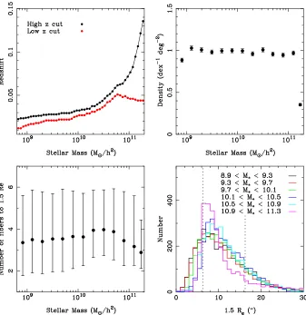
Figure 1. A demonstration of the sample selection methodology. The top left panel shows the lowest redshift interval at each stellar mass that will produce a sample of galaxies where 80% can be covered to 1.5 Reby the 127-fiber IFU (the largest available in this simulation) with a flat number density distribution as a function of stellar mass with a density of 1 deg−2
log(M∗)− 1
. The top right panel shows the resulting stellar mass distribution when these cuts are applied to the parent catalog. The bottom left panel shows the distribution of the number of 2.5′′-spaced fibers that are required to cover 1.5 R
eof each galaxy. The points show the median and the error bars show the 20th and 80th percentiles. The central fiber is not counted, i.e., the 127-fiber IFU has 6 radial fibers. The bottom right panel shows the resulting angular size distribution of 1.5 Re in bins of stellar mass. The distributions are very similar regardless of stellar mass, with the exception of the most massive galaxies. The vertical dotted lines show the radii of the 19- and 127-fiber IFUs.
K-corrections and absolute magnitudes20(using kcorrect v4 3), Sersic profile fits, and stellar masses are deter-mined.
The NSA also provides a ∼ 30% improvement in spectroscopic completeness over the standard SDSS spectroscopic catalog for the very brightest sources by adding in redshifts from the NASA Extragalactic Database (NED21), the CfA Redshift Survey (ZCAT22, Huchra & Geller 1991), Arecibo Legacy Fast ALFA Sur-vey (ALFALFA, Giovanelli et al. 2005), the 2dF Galaxy Redshift Survey (2dF Colless et al. 2001), and the 6dF Galaxy Redshift Survey (6dF Jones et al. 2009). The SDSS is 70% complete at rAB ∼ 14 and 95% complete atrAB∼16, emphasizing the importance of these other redshift sources. Assuming the incompleteness of SDSS is orthogonal to the incompleteness of the other sources,
20
K-corrections in the NSA catalog do not account for extinction explicitly, and make no attempt to apply an inclination-dependent extinction correction.
21
https://ned.ipac.caltech.edu/
22
https://www.cfa.harvard.edu/ dfabricant/huchra/zcat/
we estimate the completeness of the combined sample between 13< rAB<17 is 98.6%.
In order to achieve our primary sample design goals (radial coverage and stellar mass range), we need to tar-get massive galaxies atz >0.055. We have thus extended the NSA analysis to include galaxies with z <0.15.
We have made one further addition to the standard NSA analysis, the calculation of elliptical Petrosian mag-nitudes and profiles for all seven bands. The elliptical Petrosian method uses a set of elliptical annuli defined using an estimate of the axis ratiob/a(minor over major) and the position angleφ. Otherwise it uses the standard algorithm for Petrosian magnitudes, with the Petrosian radius rP defined as the major axis of the ellipse where
the Petrosian ratioη= 0.2, and with the aperture for the flux defined with a major-axis radius 2rP. Reis defined
as the major axis radius of the ellipse that contains 50% of the flux within 2rP. The NSA pipeline produces
containing 90% of the flux within 2rP.
We have also applied aperture corrections to the photometry, to account for the variation in point spread function between the bandpasses, particularly for GALEX. We do so by using the measured curve-of-growth to predict the aperture correction for an ideal elliptical galaxy, and applying this correction to the real data. For GALEX, these corrections can be of order 30% to 50% for galaxies with half-light radii around an arc-second; for SDSS they are always negligible.
Visual inspection of our targets during the target se-lection process revealed that the Sersic profile fitting suf-fered more catastrophic failures than the circular Pet-rosian profile calculation. A detailed comparison with the Simard et al. (2011) two component GIM2D Sersic fits further showed that the NSA’s single Sersic Re
es-timates are systematically overestimated for early-type galaxies (or galaxies with high concentrations) by up to 50% at high Sersic-n. Adding the elliptical Petrosian fit-ting maintained the stability of the circularized fits while also measuring axis ratios and position angles, and they do not show systematic differences with the two compo-nent Sersic fits. We therefore choose to use elliptical Pet-rosian Re and flux measurements throughout. Absolute
magnitudes and stellar mass in the NSA, and hence used here, are calculated assuming H0 = 100hkms−1M pc−1 withh=1.
This extended NSA is designated v1 0 1 and is publicly available as part of the SDSS data releases from DR13 onwards.
For the MaNGA selection we limit the extended NSA catalog to those galaxies that lie within the Large Scale Structure mask produced as part of the Data Release Seven NYU Value Added Galaxy Catalog (Blanton et al. 2005). This ensures that all targets fall in regions with good SDSS photometry and spectroscopic coverage, and are not close to very bright stars.
3. CONSTRUCTING THE TARGETING CATALOG Given the parent catalogs defined above, we now dis-cuss the construction of the “targeting catalog” that will define the final selection from which the MaNGA targets will be allocated. We are guided by three requirements:
• more than 80% of the sample should have a spec-ified radius (e.g. 1.5 or 2.5 Re) smaller than our
largest IFU bundle23.
• a flat distribution in the stellar mass proxy with a low-mass limit of ∼109M
⊙.
• the selection will only use cuts in redshift that de-pend on the stellar mass proxy (and one color in the case of the Color-Enhanced supplement).
A summary of the targeting catalog construction is as follows. We consider three targeting samples. The goal of the Primary sample is to provide coverage to a radius corresponding to 1.5 Re. The Color-Enhanced
supple-ment (roughly 17% of the final sample) produces a more uniform coverage inN U V −icolor as a function of mass
23
We define the radius of our hexagonal IFUs to be the radius of the circle that has the same area as the IFU.
when combined with the Primary sample to form the Pri-mary+ sample. The Secondary sample, designed to yield a sample size that is half of the Primary+ sample, covers larger radii, up to 2.5Re. For the optimization process
that we describe below we only consider the Primary and Secondary samples. The Color-Enhanced supplement, is produced by only slightly widening the Primary sample selection criteria in a color dependent way. That com-bined with its small size means that it has a negligible effect on the final sample size and S/N distributions and so the optimization based on the Primary and Secondary samples remains valid (see §4.5 for a demonstrations of this and a detailed description of the Color-Enhanced selection methodology).
After choosing the relative proportions of the sub-samples, we first adopt a desired total sky density of potential targets. This in itself requires an optimization process that balances the efficiency of allocating IFUs, the field-of-view, survey area, and the number and size of IFUs that can be constructed, and trade-offs in S/N, exposure time, spatial resolution and radial coverage. These are discussed in §3.4. Once the desired sky den-sity is defined, we derive stellar mass proxy dependent low- and high-redshift cuts that yield samples that meet the coverage criteria. These cuts are then optimized to deliver the highest S/N and spatial resolution across the targeting samples (in effect, this means that the lowest redshifts are preferred). We then “tile” the survey—a term that refers to the selection of MaNGA pointings across the sky and the allocation of IFUs to targets. This allows us to evaluate the final “observed” sample that is obtained as well as the frequency of unused or improperly allocated IFU bundles. We repeat the process multiple times under different assumptions for the target density, the minimum and maximum IFU sizes, and the distri-bution of fabricated IFU sizes to determine the optimal configuration. Further details are given below.
3.1. Selecting Upper and Lower Redshift Cuts Once the desired sky density has been set (see §3.4), we identify redshift intervals at every stellar mass where >80% of galaxies with that mass have a physical scale (either 1.5 or 2.5Re) that subtends an angular size that
fits within the largest available IFU (for discussion on the maximum IFU size, see§3.3). There are many such red-shift intervals, of course. By choosing the interval with the lowest redshift we maximize both the spatial resolu-tion (in kpc) and the S/N of the resulting sample, while maintaining both the radial coverage and density crite-ria. We impose a hard lower redshift limit of z = 0.01, designed to minimize the distance errors introduced by the local velocity field. This lower redshift limit also has the effect of limiting the main samples to stellar masses larger than ∼4×10⁸M
⊙/h2.
In practice, we bin the parent catalog into a fine grid in log stellar mass (or absolute magnitude) and redshift. For each stellar mass bin we find all the redshift ranges that produce the target density. We then find the lowest redshift range that yields a sample in which 80% of galax-ies can be covered to 1.5 or 2.5Re(for the Primary and
Table 1
The properties of Primary samples designed for differing max IFU sizes.
Max IFU Density Ngals NIF U Nplates Fraction of Median S/N per Median S/N per
size (deg−2
log(M
∗)− 1
) unused IFUs kpc2
at 1.5Re R2
e at 1.5Re
91 1.2 9008 22 474 0.14 3.8 220
127 1 9006 17 596 0.11 4.6 268
169 0.8 9005 13 802 0.14 5.2 304
217 0.8 9003 11 915 0.11 5.7 344
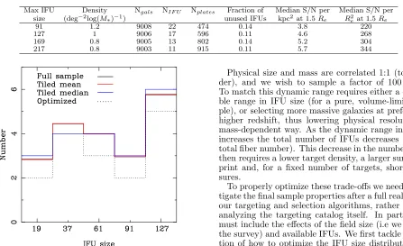
Figure 2. The required IFU size distribution to cover the primary sample to 1.5Reand the Secondary sample to 2.5Re. Galaxies smaller than 19 fibers are assigned to 19-fiber IFUs; galaxies larger than 127 fibers are assigned to 127-fiber IFUs. The solid black histogram indicates the mean size distribution of the whole sample. The red histogram shows the mean size distribution per tile after allocating IFUs using a non-overlapping tiling of the sample. The blue histogram shows the median distribution per tile. All three solid histograms have been normalized to a total of 20 galaxies. The dotted histogram is the optimal IFU size distribution that can fit on the slit. See text for the exact optimization procedure.
Figure 1 shows the results of applying this method un-der the assumption of a sky density of 1 deg−2log(M
∗)−1
and a maximum IFU size of 127 fibers. While the upper and lower redshift cuts (top left panel) may look some-what convoluted, they produce a sample that has a very similar angular size distribution across all stellar masses. This means that we probe the same spatial resolution in units of Re at all masses, although the physical
resolu-tion in kpc is mass-dependent. We will return to this point later. We note that the change in the distributions for the highest mass galaxies is unavoidable. Due to the steepness of the mass function there is a shortage of these galaxies at very low redshifts.
The bottom panels of Figure 1 also show that even in a narrow mass and redshift range the galaxies show a wide variation in size. In fact even if we were to look at a single stellar mass (or magnitude) and redshift there is still a significant range in galaxyRe(rms∼50%). Therefore, a
range in IFU sizes is required to most efficiently observe the sample.
3.2. Optimizing the IFU Size Distribution
Physical size and mass are correlated 1:1 (to first or-der), and we wish to sample a factor of 100 in mass. To match this dynamic range requires either a compara-ble range in IFU size (for a pure, volume-limited sam-ple), or selecting more massive galaxies at preferentially higher redshift, thus lowering physical resolution in a mass-dependent way. As the dynamic range in IFU size increases the total number of IFUs decreases (for fixed total fiber number). This decrease in the number of IFUs then requires a lower target density, a larger survey foot-print and, for a fixed number of targets, shorter expo-sures.
To properly optimize these trade-offs we need to inves-tigate the final sample properties after a full realization of our targeting and selection algorithms, rather than just analyzing the targeting catalog itself. In particular we must include the effects of the field size (i.e we must tile the survey) and available IFUs. We first tackle the ques-tion of how to optimize the IFU size distribuques-tion given a maximum and minimum IFU size. In the next section we will discuss how the maximum and minimum size is chosen.
Since our final sample of galaxies will have a range of apparent angular sizes (see Figure 1) we would like to have a range of IFU sizes that is able to closely match this distribution. We always wish to observe a galaxy with an IFU that is large enough to reach the desired radius, but, to maximize survey efficiency, we do not wish to use an IFU any larger. If in a given tile24 we have many more targets than available IFUs we can select the galaxies that match our IFU size distribution and thus maximize our survey efficiency. However, if the IFU distribution does not match the underlying galaxy size distribution we will produce a final sample that is biased compared to our input sample. For these reasons we want to carefully select the IFU size distribution that most closely matches the per tile size distribution derived from the targeting catalog.
Figure 2 shows the distribution of required IFU sizes for a potential targeting catalog. The construction of this catalog assumed a Primary-to-Secondary ratio of 2 to 1, a maximum IFU size of 127 fibers, and a Primary sample density of 1 deg−2 log(M
∗)−1. Galaxies that require an
IFU size smaller than 19 fibers are assigned to a 19-fiber IFU and likewise galaxies that require an IFU size larger than 127 fibers are assigned a 127-fiber IFU. The black histogram in Figure 2 shows the size distribution derived from the full targeting catalog, assuming that all
galax-24
Table 2
Optimal IFU size distributions
Max IFU size N19 N37 N61 N91 N127 N169 N217 mean square difference/dof
91 4 6 5 7 0 0 0 5584
127 2 4 4 2 5 0 0 5794
169 1 2 3 2 1 4 0 7072
217 1 2 2 1 1 1 3 6182
ies can be equally well observed. In fact, galaxies can “collide” (if a pair is closely separated only one may be allocated an IFU) and are highly clustered resulting in some regions with more or fewer available targets than MaNGA has IFUs.
After running a non-overlapping tiling of the target-ing catalog (see §5), the importance of these effects can be judged by the resulting mean (red histogram) and median (blue histogram) distributions, defined per tile. In all cases, the size distributions are scaled to a total number of 20 IFUs, which is the median number of tar-get galaxies per tile in the adopted tiling scheme. The red or blue histogram in comparison to the black his-togram represents two extreme tiling strategies. The non-overlapping tiling is the most efficient in terms of maximizing the number of galaxies observed with a given number of plates while still probing all environments, but makes no attempt at completeness. The distribution in the full targeting catalog represents 100% completeness while paying no attention to efficiency. Our eventual strategy will be somewhere between the two but we can see that there is practically no difference between the two means (black vs red).
Since we are limited to selecting integer numbers of IFUs, the blue histogram in Figure 2, the median dis-tribution of the non-overlapping tiling, looks to be a good solution. However, these IFUs would require more fibers than can fit on the slit of the BOSS spectro-graph even with our minimum acceptable slit spacing (see Drory et al. 2015). Therefore, we must find the IFU size distribution that most closely matches these required distributions but requires fewer fibers than can fit on the BOSS spectrograph slit.
To achieve this optimization we perform an exhaus-tive search over a large number of IFU size distributions where the number of IFUs of a given size varies from 0 to 8 and where the total slit space consumed is always less than the maximum available. We then calculate the mean square difference between each test IFU size dis-tribution and the actual required IFU size disdis-tribution, where both are normalized to a total number of 20 IFUs. We do this both for the full targeting catalog size dis-tribution and for each of the non-overlapping tiles. In the case of the non-overlapping tiles the mean square difference is then summed over all tiles. The best IFU size distribution is then that which minimizes the mean square difference.
For the sample described in this section the optimal IFU size distribution is 2,4,3,2,5 for both the tiled and untiled samples. It is shown as the dotted line in Figure 2. We note that a distribution of 2,4,4,2,5 is almost as good a fit and can also be accommodated on the slit. Since it wholly contains the optimal distribution but in-cludes an extra IFU it would be logical to choose this
distribution as it will yield a larger final sample that can be reduced to the optimal distribution (2,4,3,2,5) after the observations are completed, if so desired.
3.3. Selecting the Maximum and Minimum IFU Size Early work defining the survey and instrument strategy resulted in the definition of a sample that required an IFU size range from 19 to 127 fibers. This size range was determined by a combination of the requirements of the initial sample selection and the properties of the instrument and has been used for the IFU development work. In this section we revisit this choice of IFU size range and investigate if it is optimal.
3.3.1. Minimum IFU Size
The choice of the the 19-fiber IFU as the minimum possible size is a simple one. We require at least 3 ra-dial bins for all of our science cases and so smaller IFUs are not worthwhile. Our sample selection methodology (§3.1) is not directly constrained by the minimum IFU size, but instead maximizes the angular size of the sam-ple. As such, we can make the 19-fiber IFU available to our IFU size distribution optimization procedure (§3.2) and see if it is required for a given sample.
3.3.2. Maximum IFU Size
The choice of a maximum IFU size is somewhat more complex as it enters directly into the determination of the stellar mass dependent redshift cuts that define our samples (§3.1). A larger maximum IFU size will allow a sample to have a lower average redshift and still be covered to the same physical scale (e.g. 1.5 or 2.5 Re).
Clearly selecting a sample at lower redshift will improve the resolution and could potentially increase the S/N. The downside is that an increase in the IFU size reduces the total number of IFUs that will be available, since the slit length and hence number of fibers is fixed. Thus, to achieve the same sample size with fewer IFUs the number of plates observed must increase, and thus with a fixed amount of survey time available the exposure time per plate must be reduced.
We investigate these tradeoffs by designing a series of samples with different maximum IFU sizes of 91, 127, 169, 217. In each case we design Primary and Secondary samples where 80% of the galaxies are covered to 1.5 and 2.5 Re respectively by the maximum IFU size. We
choose the target densities of each sample so that when they are tiled each sample has the same fraction of IFUs that are unused due to tiles with too few targets on them. For each sample, we optimize the IFU size distribution using the procedure described in§3.2 utilizing a full non-overlapping tiling, with the results shown in Table 2.
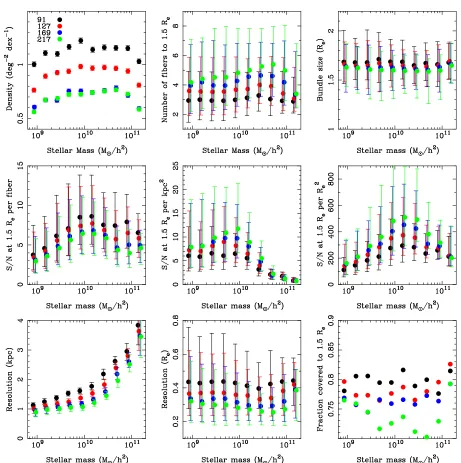
Figure 3. Performance comparison of different samples designed with different maximum IFU size. Black, red, blue, and green symbols represent samples with a maximum IFU size of 91, 127, 169, and 217 fibers, respectively. See text for detail.
the number of tiles required to produce a sample of 9,000 galaxies. For each tile, galaxies are selected to match the available IFU sizes. If there are more IFUs of a given size than galaxies of that size, they are allocated to galaxies that cannot be allocated an IFU of the correct size (see 5.3 for more details of the allocation process).
Table 1 gives some of the properties of these samples. Details of the performance of the Primary sample are shown in Figure 3. The S/N values in the table and plots are calculated using an exposure time inversely propor-tional to the required number of plates. We assume an exposure time of 3 hours for the sample designed for a maximum IFU size of 127 fibers and scale the exposure time for the other samples accordingly to ensure the same total survey time.
The top row of panels in Figure 3 simply show that the Primary samples are performing as designed. The
center row compares the S/N properties and the bottom row the resolution and coverage. We assume an effective angular resolution of 2.5′′based on expectations for the
reconstructed data cubes. The center left panel shows that the median S/N per fiber at 1.5 Re decreases as
the maximum IFU size increases. This S/N decrease is simply due to the decrease in exposure time per plate, required since we must observe more plates to achieve the same final sample size with fewer IFUs per plate. A better representation of the S/N is given by the two other panels in the center row, which show the S/N at 1.5Reper kpc2and perR2e respectively25. The opposite
25
The S/N perR2eat 1.5Reis a useful if perhaps unusual metric.
To compute it, we consider the integrated S/N in a small annulus (or fiber) positioned at 1.5Re. We then divide by the area of that
annulus in units ofR2
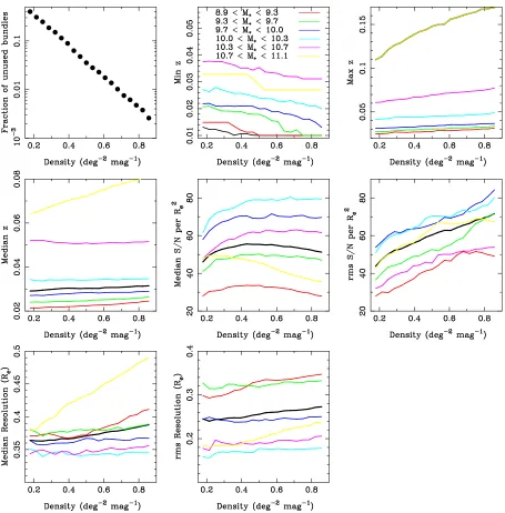
Figure 4. A comparison of key properties among samples designed with different target densities per square deg. per magnitude. The top left panel shows the fraction of unused IFUs decrease as we increase the number density of potential targets on the sky. The other panels show various properties as a function of the density. In each panel, colored lines indicate different stellar mass bins and the black line indicates the property for the whole sample. See text for more details.
trend is now apparent, with the S/N increasing as the maximum IFU size increases, since each kpc or unit of Re covers more fibers at lower redshift. This trend is
confirmed by the median S/N values for the whole of each sample given in Table 1. The largest fractional S/N increase occurs when increasing the maximum IFU size from 91 to 127 fibers, with the relative size of the increase diminishing as the maximum IFU size increases beyond 127.
As we allow larger IFUs to be considered the resolution increases as expected. Once again the biggest
improve-angle subtended byReon the sky (e.g., in arcseconds) depends on
the galaxy’s intrinsic size and its redshift. Furthermore, this S/N metric is appropriate for addressing the fidelity of measurements of both kinematics and compositional properties that scale withRe.
ment is seen when going from a maximum IFU size of 91 to 127 fibers. This trend is not surprising since we increase the radius by one fiber each time and so there is a larger fractional increase at smaller IFU sizes. What is less obvious is the strong stellar mass dependence to the gain in resolution, with the largest effect occurring at stellar masses of a few 1010M
⊙. This reflects the fact
that galaxies in this stellar mass range have the largest mean angular sizes because they are intrinsically larger than low mass galaxies, but the turnover of the mass function means higher-mass galaxies must be targeted at increasingly more distant redshifts.
The final panel (bottom right) shows the fraction of galaxies that are covered to at least 1.5 Re after tiling.
maximum IFU size increases, but a sudden fall from 169 to 217. The fraction of the IFU complement made up by the largest IFU bundle size does decrease as the max-imum allowed size increases, leading to a reduction in the fraction covered to the target radius. There are also fewer galaxies per plate for a given IFU size making it harder to match the galaxies to the IFUs. This could be mitigated with a higher density sample but there would be a subsequent loss of resolution (see§3.4 below).
While increasing the maximum IFU size from 127 to 169 will lead to some gain in S/N and resolution (it should be noted that the same effect causes both to in-crease) with a moderate loss of coverage fraction, there are some more practical disadvantages to larger IFU sizes. Since larger IFUs require more slit space, the to-tal number per plate decreases. This results in a larger number of plates required for the same sample size and hence a higher plate production cost (30% more plates
∼$100k). Furthermore, building and testing an IFU larger than the 127 fiber IFU would have required fur-ther development again increasing costs and placing the schedule at risk. We therefore settled on a final IFU size range of 19 to 127 fibers.
3.4. Choosing the Sample Density
It is possible to construct targeting catalogs meeting our science specifications with different number densities on the sky. Given that the spatial density of galaxies varies on the sky, a higher density of potential targets al-lows more efficient tiling and more efficient use of IFUs. A higher density can be achieved by widening the red-shift intervals at a given stellar mass. While the average redshift would remain roughly constant, as required by the desire for a constant angular coverage, a wider red-shift interval would result in a wider spread in angular sizes, increasing the tension between the dynamic range of galaxy sizes and the dynamic range of IFU sizes. In addition, as the desired sky density is increased, if a hard lower redshift limit (e.g. z = 0.01) is reached or there are too few massive galaxies at low-z, the average redshift must be increased, resulting in poorer spatial resolution and total S/N.
Conversely, higher density samples have the advantage of requiring fewer plates with unused IFUs allowing us to reach the desired sample size of the main samples with fewer plates. Since our total time is fixed we may increase the exposure time and thus potentially the S/N.
Overall, input samples with higher density may have a slightly higher S/N (or more galaxies) but at a poten-tial cost of lower spapoten-tial resolution and greater sample variance in both spatial resolution and S/N.
To investigate this trade off, we generate several sam-ples using the same procedure as described in §3.1 with a large range in sky density andMi as our stellar mass
proxy. These samples are then tiled using a 2,4,4,2,5 IFU size distribution and a non-overlapping tiling, adding tiles until a sample of 10,000 galaxies is reached. A Sec-ondary sample is also included which has 50% of the density of the Primary sample.
Figure 4 shows the properties of these Primary input samples constructed from targeting catalogs with vary-ing densities. The top left panel simply shows how the fraction of unused IFUs depends on density, showing a rapid decline as density increases which asymptotes to
zero at high densities as expected. Reading from left to right and top to bottom, the next three panels show the density dependence of minimum, maximum and median redshift for all galaxies (black) and split by stellar mass (color). One can see that as the density increases the minimum and maximum redshifts diverge as expected. It is also evident that the median redshift increases lit-tle, except where zmin(Mi) hits a limit which is most
evident for the highest and lowest stellar mass bins. The final four panels show the median andrmsof the S/N and resolution respectively. The S/N is determined in a fiber at 1.5 Re and is divided by the area of the
fiber in units of R2
e. Likewise the resolution is given in
units of Re. For each density the S/N is scaled by the
square root of the relative number of plates required to reach 10,000 galaxies, representing the change in plate exposure time available in a fixed duration survey. One can see that as the density is increased the median S/N begins to increase before it reaches a plateau or turns over and begins to decrease. This turnover happens most rapidly for the lowest and highest mass samples reflecting their larger changes in median redshift, which counter-acts the increased exposure time and decreases the S/N. The median resolution again shows the largest trend for the highest and lowest mass samples as it simply tracks the median redshift and thus increases (degrades) with density. In both cases the rms increases with density, reflecting the widening high and low redshift limits.
Figure 4 makes it clear that we do not wish to tar-get samples with densities>0.6 deg−2 mag−1since the S/N has either flattened off or is declining at this point while the resolution gets poorer and the scatter in both quantities increases. However, at densities below this there is a trade-off between S/N and resolution. A den-sity of 0.53 deg−2 mag−1 maximizes the overall median S/N while only reducing the median resolution by 1% over the whole sample and produces similar results for the individual stellar mass bins with the exception of the highest stellar masses. We therefore select this density for the Primary sample.
4. FINAL TARGETING CATALOGS
We have described above our procedure and optimiza-tion strategy for constructing targeting catalogs for our Primary and Secondary samples. We have decided to allow IFU sizes of 19, 37, 61, 91, and 127 fibers and a density for the Primary+ sample of 0.53 deg−2 mag−1. If we wish to have a Secondary sample of 50% the size of the Primary+ sample we would require a density of 0.37 deg−2 mag−1. This is not simply a factor of two lower than the Primary+ density since the Mi completeness
limit of the extended NSA (Equation 4 below) means that we cover a narrower Mi range in the Secondary
sample (Mi−5logh.−18) than in the Primary sample
(Mi−5logh.−19). However, we have chosen to design
4.1. Simplifying the Selection Function
Since we have elected to design samples that have flat number densities as a function of a stellar mass proxy (and are flattened in color as well in the case of the Color-Enhanced supplement) we will need to correct for this imposed selection function for any statistical analy-sis of the MaNGA sample. Since the only selection we impose is an upper and lower redshift limit as a func-tion of our stellar mass proxy (or color and mass for the Color-Enhanced supplement) we can exactly define the volume over which any galaxy in our samples could have been selected. This allows the easy calculation of a Vmax weight for every galaxy in the sample enabling the sam-ple to be corrected back to the volume limited case (see
§6.1 for details).
However, this Vmax is only perfectly defined in the case where there are no errors on the selection parame-ter (e.g. mass, magnitude, color etc). Larger errors in the selection parameter, or the combination of errors on multiple selection parameters, translates to a larger error in the weight calculation, which would then translate into errors in any derived relations defined from the MaNGA sample. This could be particularly troubling if the error in the weight ended up correlating with an interesting derived parameter from the MaNGA IFU data.
For this reason we have elected to define the Primary and Secondary samples using justMi rather than a full
estimation of the stellar mass, and the Color-Enhanced supplement usingN U V−icolor rather than an estimate of the star formation rate. This is also the reason why we have separated the Primary and Color-Enhanced sam-ples as we have, rather than making the Primary sample fully flattened in both a mass and a SFR proxy. Such a split allows the use of just the Primary sample for anal-yses that may be particularly sensitive to errors in the weights, but still enables analyses that will need better statistics in the lower density regions of the SFR-Mass plane.
Flattening the density inMirather than mass has the
disadvantage that we end up with a significant number of low mass (108−109M
⊙/h2) blue galaxies in the
sam-ple. We therefore choose to remove these by including a color dependent absolute magnitude limit at the faint end. While this does not produce a hard cut in stellar mass, it does remove most of the very low mass blue galaxies. These cuts are defined as
g−r >0.4(Mr−5logh) + 7.4 (1)
and
g−r >0.28(Mr−5logh) + 5.6 (2)
for the Primary and Secondary samples respectively, whereg−ris the k-corrected color at redshift zero.
The final simplification we make is to define the upper and lower redshift limits for the Primary and Secondary samples using a functional form rather than an interpo-lation between narrow redshift bins. This is largely done for ease of communication and reproduction and only results in a minor change in the sample properties and minimal impact on sample performance. These limits are defined by the following functional form
zlim= (A+B(Mi−5logh))(1 +exp[C(Mi−5logh−D)])
(3) with parametersA, B, CandDfor the lower and upper redshift limits of each sample given in Table 3.
Table 3
The fit parameters for the functional form (Equation 3) of theMi−5loghdependent upper and lower redshift limits
used to define the Primary and Secondary samples.
Redshift Limit A B C D Primary lower -0.056597 -0.0039264 -2.9119 -22.8476 Primary upper -0.011377 -0.0019220 -1.2924 -22.1610 Secondary lower -0.056463 -0.0048895 -1.3773 -22.3851 Secondary upper -0.048010 -0.0046639 -1.3719 -22.3225
We also include a completeness cut required as a result of the magnitude limit of the input catalog where
z <−0.9335−0.1839(Mi−5logh)−0.01222(Mi−5logh)2 −2.7668×10⁻⁴(M
i−5logh)3. (4)
4.2. Final Sample Properties
Applying our sample design procedure (§3.1) using Mi as the mass proxy, and defining Primary and
Sec-ondary samples that provide coverage to 1.5 and 2.5Re
for 80% of potential targets results in theMi dependent
redshift cuts shown in Figures 5 and 6. Applying the IFU size distribution optimization technique (§3.2) yields a preferred distribution of 2, 4, 4, 2, 5 for a total of 17 IFUs per plate. It is worth noting here that varying the target density has little effect on the optimal IFU size distribution as long as the target radius (i.e., 1.5 or 2.5 Re) and maximum IFU size remain the same. This
means that including the color enhanced sample or ad-justing our sample selection in the future, for example by changing the relative numbers of Primary and Secondary targets, will not result in a loss of efficiency or introduce a bias from the IFU allocation.
4.3. Primary Sample Properties
Figure 5 shows the properties of the Primary input sample from which actual MaNGA targets will be se-lected. The top row of panels show the redshift cuts and the density distribution as a function of bothMiand M∗.
The center left panel shows the fraction of targets that can be covered to 1.5Rewith a 127 fiber IFU and the
cen-ter panel the angular size distributions in six equal bins in stellar mass26 with vertical dashed lines showing the size of the 19 and 127 fiber IFUs. We can see from these panels that the redshift cuts are doing an excellent job of achieving the desired flatMi distribution, an
approx-imately flat M∗ distribution and an even angular
cover-age. All galaxies, irrespective of their mass, have very similar angular size distributions, meaning that they will be covered by the same range in IFU sizes. 80.1% of the sample have 1.5 Re smaller than the radius of the 127
26
We use M∗rather than Mi as it is the underlying physical
Figure 5. The selection (first three panels) and detailed properties (other panels) of the final Primary sample. Colored histograms indicate different stellar mass bins. See text for detail.
fiber IFU with just 3% requiring an IFU smaller than the 19 fiber IFU to reach 1.5 Re. The introduction of
the functional forms for the high and low redshift selec-tion cuts results in much smoother cuts at the expense of some minor variation in the density (top middle panel) and coverage fraction (center left panel).
The remaining panels of Figure 5 show distributions of scale and S/N. These are again shown in six mass bins but in these panels the vertical dotted line shows the median for the full sample. The physical resolution in kpc (center row, right panel) depends strongly on stellar mass, especially at high masses, as a result of the typical redshift increasing as the mass increases. For masses < 1010M
⊙/h2 the median resolution is 1.2 kpc, which
increases rapidly to a median of 3.85 kpc for the highest mass bin. The median for the full sample is 1.37 kpc. For the most massive galaxies (>1010.9M
⊙/h2) there is
very little hope for improving the resolution since there are so few of them at low redshifts. For galaxies with 1010< M
∗<1011there are lower redshift galaxies which
would yield higher resolutions but these are just too large to be covered to 1.5 Re. We note that some of these
galaxies will be included in an ancillary sample.
When one switches to assessing resolution in terms of Re(bottom left panel) then the sample produces
distri-butions that are almost independent of stellar mass. The median resolution for the full sample is 0.35Re.
The bottom center and right panels give an indication of ther-band S/N we can expect to achieve in a typical 3 hour exposure and how it depends on stellar mass. The bottom center panel shows the r-band S/N per fiber at 1.5Reand the bottom right panel the total S/N in an
Figure 6. The selection (first three panels) and detailed properties (other panels) of the final Secondary sample. Colored histograms indicate different stellar mass bins. See text for detail.
annulus will cover 1.35-1.8Re. The S/N is lowest for the
lowest mass galaxies and increases with mass until the highest masses, where it again decreases. These trends are simply the result of the intrinsic surface brightness distribution of the galaxy population. The medians of the S/N for the full sample at 1.5 Re are 8.3 per fiber
and 37.3 in the outer quartile annulus. Note here that the S/N refers to the spectral S/N per pixel (10−4in log wavelength in ˚A) in the r-band.
4.4. Secondary Sample Properties
Figure 6 shows the properties of the Secondary sample in the same manner as for the Primary sample above. TheMi completeness cut Equation 4 is clearly visible in
the top left panel as a diagonal cutoff in the high
red-shift selection cut at faint magnitudes. This reduces the overall range inMi and hence M∗ sampled compared to
the Primary sample, limiting the Secondary sample to M∗ > 2×10⁹. The other two plots on the top row of
the figure again show the density of targets as a function of Mi and M∗ but unlike the Primary sample there are
Figure 7. The design of the Color-Enhanced supplement. In all panels the Primary sample is shown in red, the Color-Enhanced supplement in blue and the combination (Primary+ sample) in black. The top row shows from left to right theN U V −ivs
idistribution for the Primary, the Color-Enhanced and combination of the two respectively. The Color-Enhanced supplement fills in the regions of this plane that are sparsely populated in the Primary sample. The bottom left panel shows the distribution in theMi-redshift plane for the Primary and Primary+ samples. The Primary+ sample includes galaxies at both higher and low redshifts than the Primary sample. The bottom center panel shows the density distribution of the two samples and the combination of the two, as a function of stellar mass. The roughly flat dependence of density on mass is maintained. The bottom right panel shows the median angular size of the galaxies (in units of fiber diameter) for the two samples and their combination. The error bars show the 20th and 80th percentiles. At high masses we are typically adding large galaxies with the opposite being true at small masses. The overall size distribution remains roughly unchanged when adding the Color-Enhanced supplement to make the Primary+ sample.
the MaNGA sample along side the other selection cri-teria (see §6.1). Since the required correction is well determined and barely more complex than was already required, and that we had already observed for approx-imately two years when this error was discovered, we decided that overall it was simpler to continue with this mass dependent down-sampling of the Secondary sample for the full duration of the survey.
As for the Primary sample these redshift cuts once again meet our IFU coverage target with 80.7% of the galaxies having 2.5 Re less than the radius of the 127
fiber IFU, and with just 1% having 2.5Re smaller than
the 19 fiber IFU. Again the angular size distributions are largely independent of stellar mass.
To achieve such coverage one must select a sample at higher redshift than the Primary sample. This has obvious consequences for both the resolution and S/N. The median resolution is a factor of 1.7 poorer for the Secondary sample compared to the Primary sample, al-though this is partly due to the Secondary sample being restricted to higher masses as a result of the complete-ness limits. The S/N at 2.5 Re (the edge of the IFU)
is low with a median S/N of just 2.3 per fiber and 11.4
in the outer quartile annulus. The aim of this sample is not to study continuum properties at 2.5 Re but those
of emission lines, which will naturally have much higher S/N. Even so the expected S/N in the outer annuli should be sufficient for some absorption line studies, and can be increased further by stacking multiple galaxies.
4.5. Color-Enhanced and Primary+ Samples While there are many attractive reasons to simply se-lect a sample that is flat in Mi, the resulting sample is
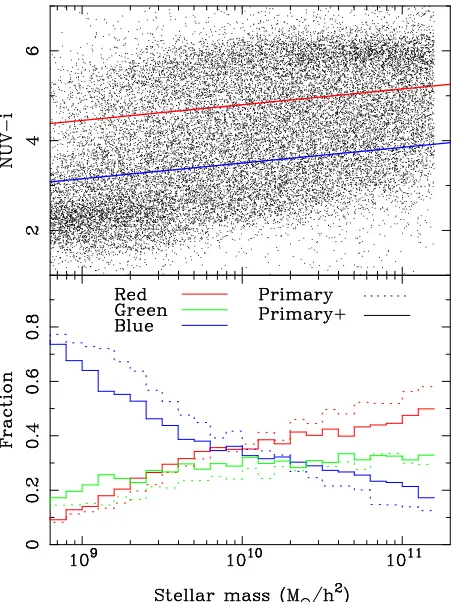
dominated by red galaxies at high masses and blue galax-ies at low masses (see Figure 8). A number of MaNGA’s primary science drivers concentrate on either red or blue (early or late type) galaxies, and we wish to study how their properties depend on stellar (or dynamical) mass. To improve the statistics for such samples we have de-signed a Color-Enhanced supplement, which increases the number of galaxies in underpopulated regions of the color (N U V−i) versus magnitude (Mi) plane. We chose
Figure 8. Top: The distribution of the Primary+ sample in theN U V −istellar mass plane. The red and blue lines are
used in the bottom panel to divide galaxies into red, green and blue. Bottom: The fraction of red, green and blue galaxies as a function of stellar mass for the Primary (dotted) and Pri-mary+ (solid) samples. The inclusion of the Color-Enhanced supplement in the Primary+ sample flattens these distribu-tions and increases the numbers of rarer galaxies.
range means that galaxies can still be better separated than if we’d usedg−ifor example. The Color-Enhanced supplement is designed to be observed to 1.5Reand will
be combined with the Primary sample to form the Pri-mary+ sample.
We construct the Color-Enhanced supplement by considering regions of the color–magnitude plane for which the number density of galaxies is < 36% of the peak density, which occurs at the luminous end of the red sequence. We calculate these num-ber densities over regions 0.1 mag wide in Mi and
0.2 mag wide in N U V −i across a range in absolute magnitude (−16.5 > Mi−5logh > −23.5) and color
(1.6 < N U V −i < 6.4). When considering the bluest and reddest color bins, we also include galaxies with N U V −i < 1.6 and N U V −i >6.2, respectively. For each bin in the color-magnitude plane we expand the redshift limits as defined by the Primary sample to include more galaxies using the following procedure:
1. We expand the redshift limits until the number density for the Primary+ sample in that bin is 36% of the peak density, or the number density is in-creased by a factor of three, or we hit the limiting redshift range of the parent catalog (0.01 < z <
0.15).
2. If fewer than 50% of the newly added color-enhanced galaxies in the bin have 1.5Re lying
within our IFU size range we reduce the redshift limits of that bin until ≥50 do have 1.5Re lying
within our IFU size range, or until half of the candi-date Color-Enhanced galaxies have been removed.
These criteria strike a balance between increasing the number density and ensuring coverage to the target ra-dius.
As for the Primary and Secondary samples we always apply a minimum redshift limit of z = 0.01 and a max-imum redshift limit below the Mi completeness limit
(Equation 4).
The demographics of the full Primary+ sample are il-lustrated in Figure 7. The top row shows from left to right the distribution in the NUV-i vs Mi plane of the
Primary, Color-Enhanced and Primary+ (the Primary plus the Color-Enhanced) samples. The Color-Enhanced selection is mainly adding galaxies in thegreen valleyand in the faint end of the red sequence and the bright end of the blue cloud. The distribution of the Color-Enhanced supplement in the redshift-Mi plane, along with that of
the Primary sample is shown in the bottom left panel and the number density of the Primary, Color-Enhanced and Primary+ samples in the bottom middle panel. The bottom right panel shows that the median angular size of the galaxies in units of fiber diameter, with the er-ror bars showing the 20th and 80th percentiles. The Color-Enhanced supplement typically adds galaxies with a smaller angular size (as a result of their higher redshift) than in the Primary sample at low masses and galaxies of a similar size, but with a slightly larger spread at higher masses. This actually results in a slight increase in the fraction of galaxies in the Primary+ sample that can be covered by the largest IFUs to 1.5 Re but a slight
de-crease in the average spatial resolution.
Figure 8 shows the performance of the Primary+ sam-ple in flattening the color-mass distribution of galaxies. The top panel shows the color-mass distribution along with two lines designed to split the sample into red-sequence, green valley and blue cloud galaxies. The bot-tom panel shows how the fraction of each of these three galaxy classes depends of stellar mass for both the Pri-mary and PriPri-mary+ samples. While there are still more low mass blue galaxies and high mass red galaxies in the Primary+ sample, the trends of red and blue fraction with stellar mass have been flattened by the addition of the Color-Enhanced supplement and the fraction ofgreen valleygalaxies increased.
5. TILING THE SURVEY
In order to execute the survey we must decide how we will cover the area spanned by the targeting catalog and allocate IFUs to potential targets. We refer to this process as tiling.
5.1. Pointing strategy
Figure 9. An illustration of two potential tiling strategies. The plot on the left shows a non-overlapping tiling and the plot on the right shows an adaptive overlapping tiling designed to produce a more even completeness irrespective of target density. The black points show the positions of galaxies in a our final Primary+ and Secondary targeting catalogs. The blue ellipses show the outlines of the tiles. The green points show those galaxies that lie within the footprint of these tiles and the red points those galaxies that were assigned IFUs
tiles are allowed to overlap, or indeed repeat, represents a trade-off between efficiency and completeness.
The left panel of Figure 9 shows the distribution of galaxies in our Primary+ and Secondary samples over the full SDSS DR7 footprint, along with an example tiling designed to have non-overlapping tiles. Looking at this figure it is apparent that the number of targets per tile varies considerably; the mean number of poten-tial Primary+ and Secondary MaNGA targets is 27.0 per tile, with anrms of 15.9, a minimum of 2, and a maxi-mum of 233.
One of our requirements is that the selection will be unbiased with respect to environment. This means that we should not choose to ignore a region where we have fewer galaxies than IFUs. It also means that we need to overlap tiles in denser regions on the sky to achieve sim-ilar completeness in dense environment as in voids. The right panel of Figure 9 shows the results of our adap-tive tiling routine. In this scheme we use a ‘gravita-tional’ method to assign multiple overlapping plates to the densest regions. The method starts with an evenly distributed overlapping tiling of∼2000 tiles. The target galaxies then ‘pull’ tiles as an 1/r2law, with the mass of already assigned targets set to zero. The velocity with which the plates are allowed to move is damped to pre-vent oscillation of the tiles and a mild repulsive force between the plates is included. This has the effect of pulling plates towards the over dense regions and away from the voids. Currently only plates with >7 targets are included in the final tiling.
This adaptive tiling scheme is highly effective at in-creasing our coverage of the densest regions without a significant loss of either IFU allocation efficiency or the ability to assign the correct size IFU to each target. The IFU allocation efficiency is 97.8% (which increases to 98.5% when the ancillary targets are included; see§5.4) and the completeness within the tiled footprint is 87% (which decreases to 85% when the ancillary targets are included), which compares well with the non-overlapping
tiling which has a 93% efficiency and a 60% complete-ness. In the adaptive scheme 93% of the galaxies are allocated IFUs matching the target size and 77% are al-located IFUs ≥ 1.5 or 2.5 Re compared to 96.7% and
78% for the non-overlapping tiling. Surprisingly we see that the overlapping tiling has an increased allocation efficiency but this is simply the result of the removal of tiles that overlap the edge of the imaging region. It also produces a slight decrease in the allocation of IFUs with the desired size. This decrease is caused by the increased completeness, resulting in a reduction in the average number of available IFUs on each tile, making it harder to find galaxies with target sizes matching the available IFU sizes.
As well as providing a more even sampling of dense environments our adaptive (overlapping) tiling scheme also enables us to improve observing efficiency. Because we have more total tiles over our area, we have more tiles in the LST regions with fewer overall tiles than in the non-overlapping case, and so can observe the easier tiles in those regions, i.e. ones that are at lower airmass and take less exposure time to complete. Our survey simulations suggest that the adaptive tiling will result in an increase of almost 10% in the total number of plates that we can complete during the survey.
5.2. Quality Control and Visual Inspection Before allocating IFUs to potential targets we under-took a set of visual inspections of the target catalog to make sure the photometry and hence selection of the tar-gets was reliable. We inspected all galaxies where there was an indication that there may be an issue with the photometry or redshift. Specifically where the Sersic and Elliptical PetrosianRediffered by a factor of 3 or more,
the Elliptical Petrosian Re >20”, the photometric and
Figure 10. The fraction of galaxies allocated an IFU (blue) and the fraction allocated an IFU of the correct size (red) as a function of stellar mass (left) andRe (right) for the Primary (top) and Secondary (bottom) samples. The dashed lines show the fraction irrespective of stellar mass or size. The open lighter colored points show the raw fractions, whereas the filled darker points show the fractions corrected using the IFU size allocation bias weight (see text for details).
Galaxies were flagged as bad where the photometry had clearly and significantly failed, due to e.g. bad imaging, bad deblending with a nearby bright start or galaxy, or a catastrophic background subtraction issue. Galaxies were also flagged where the redshift allocated clearly cor-responded to a different galaxy. Finally we provided a new center if the catalog center was obviously incorrect, mainly due to the presence of a foreground star, bright sub-region, or strong dust lanes.
To check that our preselection was catching the vast majority of issues we inspected 500 random targets not already flagged as bad finding no major photometry or centering issues. However, since we do not wish to waste an IFU as the survey proceeds we inspect the targets on each tile before we use that tile to drill any plate that will be observed, again flagging galaxies in the same way. Overall the inspection done to date we have flagged 1227 galaxies as bad and recentered 1189, each amounting to <3% of the total targets.
Finally we flag the 983 targets lying within 25′′ of
a bright star (r < 14 mag) using the APASS DR8 (Henden et al. 2012) and Tycho 2 (Høg et al. 2000) star catalogs. No targets flagged as bad or close to a bright star are eligible for IFU allocation.
5.3. IFU Allocation
Once we have broken the survey area into tiles, the next step is allocating individual IFUs to galaxies in each tile. Our method for this procedure is designed to maxi-mize the allocation of IFUs to galaxies of the appropriate size. It proceeds as follows:
1. All galaxies within a given tile are selected.
2. Galaxies that collide with the center post (within 150′′) are removed and one of every colliding pair
(within 120′′) selected at random is removed.
Figure 11. Left panels: The distribution in the number of galaxies targeted as a function of group luminosity for the Primary (top) and Secondary (bottom) sample. The solid histograms show all targets and the dotted just those allocated an IFU. We additionally divide the targets into centrals (blue) and satellites (red). Right panels: The fraction of galaxies allocated an IFU of any size (top sub panel) and with a size greater than or equal to the target size (bottom sub panel) as a function of group luminosity for the Primary (top) and Secondary (bottom). All galaxies are shown in black, centrals in blue and satellites in red as before.
2.5 Re) are selected. Galaxies with a target radius
smaller than the 19-fiber IFU are included in the 19-fiber IFU allocation (galaxies larger than the 127-fiber IFU are likewise assigned to the 127-fiber IFU).
4. All available 19-fiber IFUs are assigned to these galaxies.
5. If there are fewer galaxies that need 19-fiber IFUs than available 19-fiber IFUs, the remaining IFUs are put into a pool to be assigned later.
6. This process is repeated for the remaining IFU sizes.
7. The unassigned IFUs are then allocated to the re-maining galaxies closest in target size, beginning
with the largest galaxies and the largest remaining IFUs, and then working downwards.
Galaxies from all the main samples are treated iden-tically (i.e. none are preferred) except those Secondary galaxies that have been removed by down-sampling to get the correct relative number of Primary and Secondary targets. These randomly removed Secondaries will only be allocated an IFU if there are no available targets from another sample.