Modern Economy, 2011, 2, 213-227
doi:10.4236/me.2011.23027 Published Online July 2011 (http://www.SciRP.org/journal/me)
International Linkages of the Indian Commodity
Futures Markets
Brajesh Kumar1, Ajay Pandey2
1Jindal Global Business School, O P Jindal Global University, New Delhi, India 2Finance and Accounting Area, Indian Institute of Management Ahmedabad, Ahmedabad, India
E-mail: bkumar@jgu.edu.in, apandey@iimahd.ernet.in
Received January 6,2011; revised March 2,2011; accepted March 22,2011
Abstract
This paper investigates the cross market linkages of Indian commodity futures for nine commodities with futures markets outside India. These commodities range from highly tradable commodities to less tradable agricultural commodities. We analyze the cross market linkages in terms of return and volatility spillovers. The nine commodities consist of two agricultural commodities: Soybean, and Corn, three metals: Aluminum, Copper and Zinc, two precious metals: Gold and Silver, and two energy commodities: Crude oil and Natural gas. Return spillover is investigated through Johansen’s cointegration test, error correction model, Granger causality test and variance decomposition techniques. We apply Bivariate GARCH model (BEKK) to invest- tigate volatility spillover between India and other World markets. We find that futures prices of agricultural commodities traded at National Commodity Derivatives Exchange, India (NCDEX) and Chicago Board of Trade (CBOT), prices of precious metals traded at Multi Commodity Exchange, India (MCX) and NYMEX, prices of industrial metals traded at MCX and the London Metal Exchange (LME) and prices of energy commodities traded at MCX and NYMEX are cointegrated. In case of commodities, it is found that world markets have bigger (unidirectional) impact on Indian markets. In bivariate model, we found bi-directional return spillover between MCX and LME markets. However, effect of LME on MCX is stronger than the ef- fect of MCX on LME. Results of return and volatility spillovers indicate that the Indian commodity futures markets function as a satellite market and assimilate information from the world market.
Keywords:International Linkages, Commodity Futures Markets, Return Spillover, Volatility Spillover, Variance Decomposition Techniques, BEKK
1. Introduction
Risk management and price discovery are two of the most important functions of futures market [1-2]. Futures markets perform risk allocation function whereby futures contracts can be used to lock-in prices instead of relying on uncertain spot price movements. Price discovery is the process by which information is assimilated in a market and price converges towards the efficient price of the underlying asset. In financial economic literature, the price discovery function of futures market has been stud- ied in two broad contexts a) return and volatility spill- over between spot and futures of an asset, and b) interna- tional link-ages or return and volatility spillover across different futures markets (across countries). This paper
Empirical literature on price discovery in futures mar- kets mostly covers the relationship between futures and underlying spot prices. In equity markets, price discovery function of futures markets has been extensively studied [3-11]. In commodity futures market, price discovery function of futures markets has also been investigated [12-16]. However, these studies are mostly from devel-oped markets like US and UK. Most of the studies in equity and commodity spot-futures markets linkages confirm the leading role of futures markets in informa-tion transmission and in fore- casting future spot prices. Surprisingly, very few studies have sought to investigate the information transmission through futures prices on the same underlying, traded across different markets. In emerging commodity futures market context, interna-tional linkages of commodity futures market with devel-oped futures markets have been even less explored.
Since the inception of the organized commodity de- rivatives markets in India in 2003, Indian futures markets have grown rapidly. In 2003, three national level multi commodity exchanges, National Multi Commodity Ex- change (NMCE), Multi Commodity Exchange (MCX) and National Commodities and Derivatives Exchange (NCDEX), were setup. At present, commodity futures are traded on three national exchanges, and 20 other re- gional exchanges, which have been in existence for longer time. Currently, the futures contracts of around 103 commodities are traded on three national exchanges. In terms of volume, Copper, Gold, Silver and Crude fu- tures traded on Multi Commodity Exchange (MCX), India has been ranked within the top 10 most actively traded futures contracts1 in the world. However, the
commodity futures markets in India are subject to many regulations and many a times have been criticized for speculative trading activity as well as for causing an in- crease in spot price volatility [17]. Emerging commodity markets are generally criticized for speculative activity and destabilizing role of derivatives on spot market through increased price volatility [16,18,19].
Most of the studies on Indian commodity futures mar- kets are limited to policy related issues. Some of the ma- jor issues identified and investigated in Indian commod- ity futures are: the role of spot markets integration and friction (high transaction cost), proper contract design, identification of delivery location, importance of ware- housing facilities and policy issues like restriction on cross-border movement of commodities, different kind of taxes etc [20-22]. The literature on price discovery on
Indian com- modity futures markets is limited to regional exchanges, dated/small sample form the period prior to setting up of national exchanges, or to very fewer com-modities traded on national exchanges [23-26]. The In-dian commodity futures markets have since then matured and have started playing a significant role in price dis-covery and risk management in the recent period, if in-creased volume of trading is any indicator. Trade and financial liberalization in the country and rest of the world may also have led to strong integration of Indian markets with their world counterparts. However, the re-lationship between the Indian and world commod- ity futures markets has not been explored adequately and hence there is a case for investigating the linkages of Indian commodity futures markets with the counterparts elsewhere in the world trading the futures contracts on the same underlying.
2. Literature Review
The research on international linkages across markets has been mainly on the financial asset markets [27-34]. Eun and Shim [23] found the dominance of US equity market in information dissemination to rest of the world. They found that any innovations in the US equity futures mar-ket are rapidly transmitted to other marmar-kets, whereas no single foreign market can significantly explain US mar-ket movements. Koutmos and Booth [30] investigated the dynamic interaction across three major stock markets New York (S&P 500), London (FTSE 100) and Tokyo (Nikkie 225) and found significant price spillovers from New York to London and Tokyo and from Tokyo to London market. Susmel and Engle [29] investigated the return and volatility spillovers between US and UK eq-uity markets but did not find strong evidence of return and volatility spillovers between these two while the studies cited above examined cross-market linkage where the underlying differed. Tse [23] investigated the Eurodollar futures markets in Chicago, Singapore, and London and found that all these markets are cointegrated by a common factor. Booth et al. [31] found that Nikkei 225 Index futures that are traded in Singapore, London and Chicago are cointegrated.
In commodity futures context, Booth and Ciner [35] investigated the return and volatility spillovers of corn futures between the CBOT and the Tokyo Grain Ex- change (TGE). They found significant return and volatil- ity spillovers between the two markets. Booth, Brockman, and Tse [33] studied the wheat futures traded on the Chi-cago Board of Trade (CBOT) of US and the Winnipeg Commodities Exchange (WCE) of Canada and found one way information spillover from CBOT to WCE. Low, Muthuswamy, and Webb [36] examined the futures
1Leading commodity futures contracts in terms of volume are Gold, Crude, Natural gas, and Silver futures traded at NYMEX in US, Alu-minum, Copper, and Zinc futures traded at LME, London, and Corn, Soybean contracts at CBOT in US. (Details:
B. KUMAR ET AL. 215
prices for storable commodities, soybeans and sugar, which are traded on the TGE and the Manila Interna- tional Futures Exchange (MIFE), and found no co-inte- gration between these two markets. Lin and Tamvakis [37] examined the information transmission mechanism and price discovery process in crude oil and refined oil products traded on the New York Mercantile Exchange (NYMEX); and London’s International Petroleum Ex-change (IPE). They found substantial spillover effects between two markets where IPE morning prices seem to be considerably affected by the closing price of the pre-vious day on NYMEX. Holder, Pace and Tomas III [38] investigated the market linkage between US and Japan for Corn and Soybean futures. They considered Corn and Soybean futures traded on the Chicago Board of Trade (CBOT) in US and the Tokyo Grain Exchange (TGE), and the Kanmon Commodity Exchange (KCE) in Japan. They found that trading at CBOT had very little effect on the Japanese contract volumes. Xu and Fung [39] inves-tigated the crossmarket linkages between US and Japan for precious metals futures: Gold, platinum, and Silver. They applied bivariate asymmetric ARMA-GARCH model to estimate the return and volatility spillovers be-tween these two markets and found that there was a strong linkage between these markets with US market playing a leading role in return spillover. They, however, found bidirec- tional volatility spillover between the two markets. Kao and Wan [40] studied the price discovery process in spot and futures markets for Natural gas in the US and UK using a quadvariate VAR model. They found that all spot prices and futures prices were driven by one common factor. They found that the US futures market dominated over UK futures market and acted as the cen-ter for price discovery. They also concluded that the spot markets in the US and UK were less efficient than their corresponding futures market.
In the emerging markets context, Fung, Leung and Xu [41] examined the information spillover between US futures markets and the emerging commodity futures market in China for three commodity futures: Copper, Soybean, and Wheat. They used VECM-GARCH model and found that for Copper and Soybean, US futures market played a dominant role in transmitting informa- tion to the Chinese market. However, in the case of Wheat, which is highly regulated and subsidized in China, both markets were highly segmented. Hua and Chen [42] investigated the international linkages of Chi-nese commodity futures markets. Commodities con- sidered in the analysis were: Aluminium, Copper, Soy- bean and Wheat. Aluminum and Copper futures traded on LME and Soybean and Wheat futures traded on CBOT were analyzed. They applied Johansen’s cointe- gration test, error correction model, and Granger
causal-ity test and impulse response analyses to understand the relationship. They found that Aluminum, Copper and Soybean futures prices are integrated with spot prices but did not find such cointegration for wheat spot and futures prices. They concluded that LME had a bigger impact on Shanghai Copper and Aluminium futures and CBOT had a bigger impact on Dalian Soybean futures. Ge, Wang and Ahn [43] investigated the linkages between Chi- nese and US cotton futures market. They considered the futures prices of contracts trading on New York Board of Trade (NYBOT) in US and the Zhengzhou Commodity Exchange (CZCE) in China. They found that these mar- kets were cointegrated and that there was bidirectional causality in returns between these markets.
To summarize, most studies on international linkages across futures markets of the same underlying suggest that there are stronger international market linkages in highly traded commodities as compared to relatively less traded commodities. Moreover the developed markets (in terms of volume and number of derivatives products) play dominant role in price discovery process. Given limited research on international linkages of futures markets in emerging markets, which are characterized by low liquidity, and exhibit higher price variability and poor information processing [44,45], this paper is an attempt to investigate the cross-market link- ages of Indian com-modity futures market with developed world futures markets for both high tradable (precious metals) and less tradable (agricultural) commodities.
China, Japan, Germany and Russia. India is among top 20 major producers as well as consumers of Aluminium, Copper and Zinc.
Given this background, firstly we test that whether In- dian commodity futures market is cointegrated with rest of the world in the long run and if so for which com- modities (tradable/less tradable)? We expect that because of the importance of Indian market in the world and also due to world trade liberalization, Indian markets should be cointegrated with rest of the world for industrial met- als, precious metals and energy commodities. It may be possible that prices are cointegrated in the long run but deviate in the short run. Hence, we further investigate whether there is any lead-lag relationship between Indian market and their world counterpart in terms of return spillover. Further, we examine the direction and speed of information transmission between the markets through return spillover. We also investigate whether there are any differences across commodities as far as return spillover is concerned. The information spillover or the market linkages are also examined by examining the second moment or volatility spillover across markets with the objective of investigation being similar to return spillover.
3. Data and Time Series Characteristics of
Returns
To examine the international linkages of Indian com- modity futures markets, we use data set consisting of two agricultural commodities: Soybean, and Corn, three met- als: Aluminum, Copper and Zinc, two precious metals:
Gold and Silver, and two energy commodities: Crude oil and Natural gas. For agricultural commodities daily prices of near month futures contracts from NCDEX and for non-agricultural commodities daily prices of near month futures contracts traded on MCX are used. The selection of a particular Indian exchange is based on trading volume of the commodity futures contract. We chose Gold, Silver, Brent crude oil, and Natural gas fu- tures price traded on New York Mercantile Exchange (NYMEX), Aluminium, Copper and Zinc futures con- tracts traded on the London Metals Exchange (LME), Soybean and Corn futures contracts traded on the Chi- cago Board of Trade (CBOT) as the counterpart markets for Indian futures markets. These are the leading ex- changes for the respective commodity futures contracts in terms of volume traded. Details of the data period and source of data are given in Table 1.
We construct the continuous futures price series using daily closing futures prices of near month futures con- tracts for all commodities. For consistency, we converted all data into USD2/unit. The Gold price is converted into USD/10grams3, Silver, Aluminium, Copper and Zinc
into USD/kg Soybean and Corn into USD/100kg, Crude into USD/Barrel and Natural gas into USD/mmBtu. The daily futures returns are constructed from the futures price data as log(Ps,t/Ps,t-1), where Ps,t is the futures price
at time t. Standard unit root test is performed on log prices and returns series. The augmented Dickey-Fuller (ADF)4
[image:4.595.54.540.490.682.2]indicates that the log prices for all commodities and in all markets have unit root and returns series are stationary. It indicates that the log prices follow an I(1) process, which is a prerequisite for the cointegration analysis.
Table 1. Details of Commodity, Data Period and Source.
Commodities Data-Period World Futures Market Indian Futures Market
Soy Bean 9/1/2004 to 1/11/2008 CBOT, US NCDEX Agricultural
Corn 1/5/2005 to 1/11/2008 CBOT, US NCDEX
Gold 5/5/2005 to 4/7/2008 COMEX, US MCX Bullion
Silver 5/5/2005 to 4/7/2008 COMEX, US MCX
Aluminium 2/2/2006 to 7/31/2007 LME, UK MCX
Copper 7/4/2005 to 7/31/2007 LME, UK MCX Metals
Zinc 8/1/2006 to 7/31/2007 LME, UK MCX
Crude Oil 5/5/2005 to 4/7/2008 NYMEX, US MCX Energy
Natural Gas 8/7/2006 to 4/7/2008 NYMEX, US MCX
2We used the daily exchange rate to convert Indian currency Rupees into US. The exchange rate data for the required period is collected from Reserve Bank of India (Federal).
B. KUMAR ET AL. 217
t
4. Long-Run and Short-Run Relationship in
Futures Prices Traded on Indian
Commodity Futures Markets and their
World Counterparts
4.1. Johansen Cointegration Test
As a first step to understand relationship between Indian commodity futures markets with their world counterparts, we test co-integration between Indian commodity futures market and international futures market. Cointegration theory suggests that two non-stationary series having same stochastic trend, tend to move together over the long run [46]. However, deviation from long run equilib-rium can occur in the short run. The Johansen full infor-mation multivariate cointegrating procedure [47,48] is widely used to perform the cointegration analy- sis. It can only be performed between the series having same degree of integration. Johansen Cointegration test can be conducted through the kth order vector error correc- tion
model (VECM) represented as
1
1 1
1
k
t t i t
i
Y Y Y
(1)Where, Yt is (n × 1) vector to be examined for cointegra- tion, ΔYt = Yt – Yt-1, ν is the vector of deterministic term
or trend (intercept, seasonal dummies or trend), П and Ѓ
are coefficient matrix. The lag length k is selected on minimum value of an information criterion5. The exis-
tence of cointegration between endogenous variable is tested by examining the rank of coefficient matrix П. If the rank of the matrix П is zero, no cointegration exists between the variables. If П is the full rank (n variables) matrix then variables in vector Yt are stationary. If the rank lies between zero and p, cointegration exists be- tween the variables under investigation. Two likelihood ratio tests are used to test the long run relationship [44].
a) The null hypothesis of at most r cointegrating vec- tors against a general alternative hypothesis of more than r cointegrating vectors is tested by trace Statistics.
Trace statistics is given by
1
trace n ln 1
i i r
T
(2)where T is the number of observations and λ is the ei- genvalues.
b) The null hypothesis of r cointegrating vector against the alternative of r + 1 is tested by Maximum Eigen value statistic
Maximum Eigen Value is given by
max
Tln 1
r1In our test for the cointegration between Indian com- modity futures market and their world counterpart, n = 2 and null hypothesis would be rank = 0 and rank = 1. If rank = 0 is rejected and r = 1 is not rejected, we conclude that the two series are cointegrated. However, if rank = 0 is not rejected, we conclude that the two series are not cointegrated.
Since all the time series of logged futures prices are I(1) series, we test the cointegration between futures prices of contracts traded in Indian commodity market and their counterpart futures exchanges elsewhere in the world. Both λtrace and λmax statistic are used to test the
cointegration. The results of the cointegration test are presented in Table 2. It is found that all commodities traded on Indian commodity futures market are cointe- grated with their world counterparts. We reject the null hypothesis of rank = 0 and can not reject the null hy- pothesis of rank = 1 for all commodities under investiga- tion at 5% significance level. It is interesting to note that futures prices of agricultural commodities (Soybean and Corn) traded on India commodity futures exchanges are cointegarted with CBOT futures prices. Hua and Chen [38] investigated the similar relationship for Chinese commodity futures market and found the long run coin- tegration with world futures market for Aluminium, Cop-per and Soybean but did not find cointegration for Wheat futures traded on CBOT and the Chinese com- modity futures exchange.
4.2. Weak Exogeneity Test
The weak exogeneity test measures the speed of adjust- ment of prices towards the long run equilibrium rela- tionship. If the two price series are cointegrated in long- run, then the coefficient matrix П (explained in Equation 1) can be decomposed as П = αβ′, where β contains cointegrating vectors and α measures the average speed of adjustment towards the long-run equilibrium. The larger the value of α, the faster is the response of prices towards the long-run equilibrium. If prices do not react to a shock or value of α is zero for that series, it is said to be weakly exogenous. We test the weak exogeneity of Indian commodity futures prices and world futures prices for each commodity. It is tested through likelihood-ratio test statistics with null hypothesis as αi= 0. The results of
this test are presented in Table 3.
The results of weak exogeneity test of Indian and the world commodity futures prices indicate that in most of the commodities, except Copper, Zinc and Natural gas, Indian commodity futures prices respond to any price discrepancies from long run equilibrium whereas the world futures prices are exogenous to the system. In case of Copper, both LME and Indian futures prices are ex-
(3)ogenous to the system. In case of Zinc and Natural gas, LME and NYMEX market respond to the error correct- ing terms to restore long run equilibrium whereas the Indian market is exogenous. Our results that the response of Indian commodity futures markets not to deviate too far from the long-run equilibrium relationship and the weak exogeneity of world prices for most of the com- modities, indicate the leading role of world market in price discovery and satellite nature of Indian commodity futures markets.
4.3. Short Run Cointegration
After examining the long run integration between Indian
and world markets, we also analyze the short-run inte- gration or return spillover between these markets. The short run integration between Indian futures prices and their world counterparts is investigated through VECM model as these prices are cointegrated in the long run. The Granger causality test is also applied to examine the lead-lag relationship between Indian and the World counterpart. We apply forecast error variance decompo- sition for each returns series to understand the economic importance of one market on the other.
Vector Error Correction Model (VECM)
[image:6.595.59.539.271.478.2]Since futures prices traded in Indian market and their
Table 2. Johansen cointegration test results.
Commodity Lag length Cointegration Rank Test Using Maximum Eigenvalue Cointegration Rank Test Using Trace
H0: rank = 0 Vs H1: rank = 1
H0: rank = 1 Vs H1: rank = 2
H0: rank = 0 Vs H1: rank = 1
H0: rank = 1 Vs H1: rank = 2
Soy Bean 3 31.7744* 2.4626 30.546* 2.1009 Agricultural
Corn 1 19.7004* 2.2961 21.0072* 2.507
Gold 4 17.8351* 5.3996 23.4629* 4.9913 Bullion
Silver 3 14.7067* 4.6723 19.379* 4.6723
Aluminium 5 24.4747* 3.8698 28.3445* 3.8698
Copper 4 13.1998* 4.9158 21.7399* 5.4253 Metals
Zinc 4 20.5895* 2.6857 29.6307* 2.5211
Crude Oil 3 17.586* 3.2128 23.2074* 3.5273 Energy
Natural Gas 3 22.6747* 2.7698 34.1376* 4.7614
* denotes rejection of null at 5% level.
Table 3. Results of weak exogeneity test.
World Prices Indian Prices
Commodity Chi-Square Chi-Square
Agricultural Soy Bean 0.87 27.65**
Maize 0.1 17.13**
Bullion Gold 0.78 3.87*
Silver 1.45 4.39*
Metals Aluminium 0.24 17.64**
Copper 1.98 1.16
Zinc 4.03* 1.64
Energy Crude Oil 2.7 3.64*
Natural Gas 23.76** 0.06
*
[image:6.595.56.540.517.706.2]B. KUMAR ET AL. 219
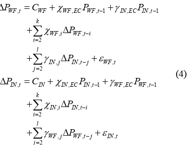
, 1
, 1
world counterparts are cointegrated, short run relation- ship (return spillover) can be examined through error correction model. Vector error correction model specifi- cations allow a long-run equilibrium error correction in prices in the conditional mean equations [46]. Similar approach has been used to model short run relationship of cointegrated variables [44-51]. The VECM specifica-tion for Indian futures prices and the world futures prices can be represented by
, , , 1 , , ,
2
, , , 2
, , , 1 ,
, , 2
, , , 2
WF t WF WF EC WF t IN EC IN t k
WF i WF t i i
l
IN j IN t j WF t j
IN t IN IN EC IN t WF EC WF t k
IN i IN t i i
l
WF j WF t j IN t j
P C P P
P
P
P C P P
P P
(4)Where, PIN,t is the log price in the Indian commodity futures market and PWF,tis the log futures prices in the
World market. The error correction termIN EC IN t, P , 1 , , 1
WF EC WF tP
or WF EC WF t, P , 1 IN EC IN t, P , 1 (П = αβ′
representation) represents the speed of adjustment to- wards long run equilibrium. The short run parameter estimates χIN,χWF, γIN and γWF measure the short run inte-
gration or return spillover. The significance and value of these parameters measures the short run spillover be- tween these markets. We performed the Granger causal- ity test to find the lead-lag relationship between Indian commodity futures prices and the World counterparts. It tests whether, one endogenous variable (say PIN,t) is sig-
nificantly explained by other variable (say PWF,t). More
specifically, we say that PWF,t Granger causes PIN,t if
some of the γWF (i) coefficients ( ) are non- zero and/or γWF,EC is significant at conventional levels.
Similarly PIN,t Granger causes PIN,t t if some of the γIN (i)
coefficients ( ) are nonzero and/or γIN,EC is
significant at conventional levels.
2,3,
i
2, ,
i p
,p
[image:7.595.98.290.192.339.2]
Table 4 represents the results of VECM for Indian commodity futures prices and their world counterpart for all commodities. As mentioned earlier, we used Akaike Information Criterion (AIC) to select the lags in the VECM. We found that error correcting terms
, , 1 , , 1
IN EC IN tP WF EC WF tP
in the equation of Indian futures prices are significant at 5% level for all com- modities except Copper, Zinc and Natural gas. In case of Copper, error correcting term in the equation of the world futures returns are not significant. These terms are however significant only for Zinc and Natural gas. These
findings are consistent with the results of weak exogene- ity tests. It can be concluded that even though Indian futures market are cointegrated with the world futures prices for Copper, Zinc and Natural gas, in the short run Indian futures markets do not respond to the error cor- recting term. However, world prices (LME and NYMEX) returns respond to the error correcting term.
These results may be biased because of small sample size for Zinc and Natural gas contracts, as these have been traded only since August 2006 in Indian market. Further, it is not clear that whether results are due to fric- tions in the Indian commodity futures markets for these commodities, or dues to high transaction cost or the leading role of Indian markets in price discovery. This is beyond the scope of the paper and further research is required to address this issue. The short run coefficients
γWF(i), which measure the return spillover from world
market to Indian futures market are also significant for Gold, Silver, crude, and Zinc. However, short run coeffi- cients γIN (i), which measures the return spillover from
Indian market to the World markets, are significant only for metals. The results of the VECM indicate bi-direc- tional causality between Indian market and their world counterparts for industrial metals. We estimated the Chi square statistics for Granger causality test to understand the lead-lag relationship between Indian commodity fu- tures returns and their world counterpart. Results of the Granger causality test are reported in the Table 5.
The results of Granger causality test indicate that for Soybean, Corn, Gold, and Silver, world futures prices lead the Indian market and affect the Indian futures re- turns. The weak exogeneity test and results of error cor- rection model also indicate the same for these commode- ties. World futures price lead Indian markets in price discovery process and Indian market respond to long run as well as short run deviations in the prices. After com- bining the results of cointegration test and VECM model, it can be concluded that for Soybean, Corn, Gold, and Silver, the world markets affect Indian futures prices both in the long and short run.
Table 4. Parameter estimates of VECM.
A. Indian Futures Prices
Commodity CIN γWF,EC χIN,EC γWF,1 γWF,2 γWF,3 χWF,4 χIN,1 χIN,2 χIN,3 χIN,4 Soy Bean 0.0910** 0.0442** –0.0553** 0.0730 0.0481 –0.0467 –0.0117
Maize 0.1487** 0.0320** –0.0530**
Gold 0.0347* 0.1897* –0.1931* 0.5358** 0.2814 –0.1374 –0.5616** –0.3062 0.2033
Silver 0.0459* 0.1190* –0.1230* 0.2774* 0.2514 –0.2996* –0.3568*
Aluminium 0.3530 0.2998** –0.3732** –0.1104 –0.0390 –0.0407 0.0469 0.2208* 0.0551 0.0401 –0.0614
Copper –0.0232 0.0937 –0.0892 –0.0356 –0.1621 –0.0884 0.0343 0.0794 0.2541*
Zinc 0.0677 0.3076 –0.3206 –0.3452 –0.3615* –0.2671* 0.5251* 0.2055 0.3801*
Crude Oil –0.0154 0.0646* –0.0624* –0.0260 –0.0817 –0.0138 0.0597
Natural Gas 0.0011 –0.0062 0.0060 –0.0167 –0.0070 0.0558 –0.1307*
B. World Futures Prices
Commodity CWF χWF,EC γIN,EC χWF,1 χWF,2 χWF,3 χWF,4 γIN,1 γIN,2 γIN,3 γIN,4 Soy Bean 0.0188 0.0086 –0.0108 –0.0205 0.0075 0.0004 0.0367
Maize –0.0148 –0.0036 0.0059
Gold 0.0182 0.0946 –0.0962 0.1239 0.0965 –0.2536 –0.1250 –0.1078 0.2936
Silver 0.0300 0.0753 –0.0779 –0.1104 0.1439 0.0893 –0.2419
Aluminium 0.0328 0.0277 –0.0345 –0.3393** –0.2279** –0.0934 0.3878** 0.1446 0.0601 0.0369 –0.1342*
Copper 0.0313 –0.1114 0.1061 –0.6304** –0.4394** –0.1985** 0.6881** 0.5084** 0.3961** Zinc –0.0956* –0.4314* 0.4496* –0.5170** –0.4100** –0.3027** 0.7920** 0.3641* 0.4998**
Crude Oil 0.0192 –0.0675 0.0652 –0.4925** –0.3081** 0.3663** 0.2194**
Natural Gas 0.0603** –0.4525** 0.4387** –0.6546** –0.3420** 0.3285 0.3447 ** and * denote significance of parameter at 1% (5%) level.
Table 5. Results of granger causality test.
International → India India → International
Agricultural Soy Bean 40.12** 1.08
Maize 16.36** 0.06
Bullion Gold 26.98** 6.43
Silver 14.02** 5.53
Metals Aluminium 21.6** 51.24**
Copper 3.83 117.79**
Zinc 6.37 152.69**
Energy Crude Oil 6.12 39.3**
Natural Gas 2.63 33.04**
[image:8.595.54.540.538.709.2]B. KUMAR ET AL. 221
they may assimilate information from US markets, which are open at that time. Our result may be reflective of this fact6. In case of energy commodities (Crude and Natural
gas), results of Granger causality test indicate that Indian futures prices lead the NYMEX prices. This again is sur-prising.
Sims [52,53] and Abdullah and Rangazas [54] sug-gested that the variance decomposition of the forecast error is advisable while analyzing the dynamic relation- ship between variables because it may be misleading to rely solely on the statistical significance of economic variables as determined by VAR model or Granger cau- sality test. Therefore, we also estimate the variance de- composition of the forecast error of each endogenous variable in order to further investigate the relationship between Indian and the world commodity futures markets.
4.4. Variance Decomposition
The variance decomposition of the forecast error gives the percentage of variation in each variable (e.g. Indian commodity futures returns) that is explained by the other variables (futures returns of markets elsewhere on the same underlying). We estimated the orthogonal variance decomposition of forecast error up to 20 lags from the VECM (Equation 4). Results of the variance decomposi- tion for Indian commodity futures returns and their world counterparts are shown in Table 6. Panel-A of Table 6
explains the percentage of variation in futures price traded on world market explained by its own lagged re- turns and futures returns traded on Indian market whereas Panel-B of Table 6 represents the percentage of
variation in Indian commodity futures returns explained by its own lagged returns and their world counterparts. As shown in Table 6, it is found that in the case of Soy- bean, Corn, Gold and Silver, variation in world futures returns are explained by their own lagged returns, whereas Indian futures returns explain 0% - 1% variation in the futures returns of the market elsewhere.
[image:9.595.49.540.491.698.2]On the other hand, in case of precious metals (Gold and Silver), variation in Indian futures returns are mostly explained by NYMEX returns (more than 90%) and its own lagged returns explain only 10% variation. In case of agricultural commodities (Soybean and Corn), CBOT returns are able to explain more than 20% [Soybean more than 20% and Corn more than 50%] of variation in Indian futures returns. Results of agricultural commode- ties and precious metals are consistent with the results of error correction model results and Granger causality test. In case of industrial metals, it is found that LME returns are able to explain more than 70% variation in Indian metals futures [Aluminium, Copper and Zinc > 70%] whereas Indian returns are able to explain more than 5% (Aluminium 5% and Copper and Zinc 20%) in LME metals futures returns. This result is not consistent with the results of Granger causality test especially results of Copper and Zinc where we find that Indian returns Granger cause LME returns. Thus, combining the evi- dence from both tests, it can be concluded that there may be bidirectional causality between Indian and LME re- turn for metals but the effect of LME on the Indian prices is stronger than the effect of Indian prices on LME prices. In case of crude, NYMEX returns are mostly explained by their own lagged returns, however Indian futures re-
Table 6. Forecast error variance decompositions.
A. World Futures return explained by B. Indian Futures return explained by
World Returns India Returns World Returns India Returns
1 5 10 15 20 1 5 10 15 20 1 5 10 15 20 1 5 10 15 20
Soy Bean 100% 100% 100% 100% 100% 0% 0% 0% 1% 1% 1% 4% 11% 19% 28% 99% 96% 89% 81% 72%
Maize 100% 100% 100% 100% 100% 0% 0% 1% 2% 2% 11% 24% 35% 45% 54% 89% 76% 65% 55% 46%
Gold 100% 100% 100% 99% 99% 0% 0% 0% 0% 0% 92% 98% 99% 99% 99% 8% 2% 1% 1% 1%
Silver 100% 100% 99% 98% 98% 0% 0% 0% 0% 0% 89% 96% 98% 99% 99% 11% 4% 2% 1% 1%
Aluminium 100% 93% 96% 97% 97% 0% 7% 4% 3% 3% 23% 47% 63% 71% 76% 77% 53% 37% 29% 24%
Copper 100% 80% 79% 80% 80% 0% 20% 21% 20% 20% 59% 60% 64% 68% 70% 41% 40% 36% 32% 30%
Zinc 100% 72% 77% 80% 81% 0% 28% 23% 20% 19% 63% 65% 73% 77% 79% 37% 35% 27% 23% 21%
Crude Oil 100% 92% 91% 90% 89% 0% 8% 9% 10% 11% 6% 4% 4% 4% 4% 94% 96% 96% 96% 96%
Natural Gas 100% 90% 78% 69% 60% 0% 10% 22% 31% 40% 45% 49% 55% 60% 64% 55% 51% 45% 40% 36%
turns are able to explain only 8% - 10% variation in NY- MEX returns. Further, NYMEX crude returns are able to explain only 4% - 6% variation in Indian returns. In case of Natural gas, Indian returns are able to explain 30% - 40% variation in NYMEX returns and NYMEX returns explains 50% - 60% variation in Indian returns. We may conclude that in case of energy commodities bidirec- tional causality exist between MCX, India and NYMEX, US. However, effect of NYMEX market on Indian mar- ket is stronger than the effect of Indian market on NY- MEX.
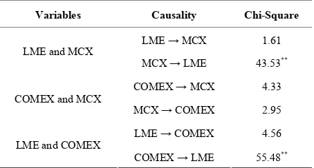
In order to shed more light into bidirectional causality between LME and MCX for industrial metals, we intro- duce a variable, COMEX, US, prices (Copper)7, in
VECM model as another endogenous variable. As ex-plained earlier, results of bivariate models with LME and MCX prices may be misleading because of extended trading period in Indian market and closing timing dif-ference between LME and Indian market. The Indian market closes around two hours after the LME market and at that time COMEX market is trading. It is likely that the information is coming from COMEX market and is affecting LME market through MCX. Trading timings of LME, India and COMEX market are given in Table 7.
First, we test the cointegration8 between LME, MCX
and COMEX Copper prices and it is found that these prices are cointegrated with single stochastic term, which indicates that the Copper prices are driven by a common factor. Results of Granger Causality test indicate that, LME prices are affected by both MCX and COMEX prices. We do not find any Granger causality between COMEX and MCX Copper futures prices. Results of Granger causality test of Copper is reported in Table 8.
We also estimate the variance decomposition from VECM (3), which explains the percentage of variation in each variable (e.g. LME copper futures returns) that is explained by other variables (COMEX copper futures returns and MCX copper futures returns) in the system. The results are shown in Table 9.
It is clear from the variance decomposition results that the LME returns’ variance is mostly explained by its own lags (65%) and COMEX returns (35%). Indian market is not able to explain any variation in the LME returns or COMEX returns. It is also interesting to see that MCX Copper return variance is mostly explained by LME (55%) return variance and COMEX return variance (38%). It indicates that even in case of metals, Indian market gets information from world markets; LME and COMEX, and Indian market does not affect LME market. This negates the results of bivariate case wherein bidi-
rectional causality between LME and Indian futures prices is found. To sum up, it can be concluded that for all commodities, price discovery takes place in the world market and Indian futures market assimilate information through return spillover.
The VECM, Granger Causality test and variance de- composition examine the information transmission be- tween markets by investigating first moment (mean re- turn). However, the information transmission is better tested by examining the second moment or volatility spillover across markets. Ross [55] demonstrated that the rate of information transmission is critically linked to volatility.
4.5. Volatility Spillover: A BEKK Model Approach
After the seminal work of Engle, Ito and Lin [56], who applied multivariate GARCH model in estimating vola- tility spillover between US and Japanese foreign ex- change markets, multivariate GARCH model has been widely applied to equity, exchange, bond and commodity markets etc. In this paper we apply multivariate GARCH model, BEKK (developed by Baba, Engle, Kraft and Kroner, 1991), to investigate volatility spillover between Indian commodity futures prices and their world coun- terpart. The residuals t
1t, 2t from VECM [image:10.595.309.537.466.549.2](Equation 4), which has conditional multivariate normal distribution the, are used in the following bivariate
Table 7. Trading timings of LME, India and COMEX ex-changes.
Exchange Timings
LME MCX COMEX
Winter 17:20 p.m. - 22.30 p.m. 10:00 p.m.- 23.55 p. m 18:40 p.m. - 23.30 p.m.
Summer 16:20 p.m. - 21:30 p.m. 10:00 p.m. - 23.00 p. m 17:40 p.m. - 22:30 p.m.
Table 8. Results of granger causality test of copper from VECM (3).
Variables Causality Chi-Square
LME → MCX 1.61 LME and MCX
MCX → LME 43.53** COMEX → MCX 4.33 COMEX and MCX
MCX → COMEX 2.95 LME → COMEX 4.56 LME and COMEX
COMEX → LME 55.48** 7We are not able to get the data of other two industrial metals. However
results of Copper can be extended to other industrial metals.
8Results of Cointegration and weak exogeneity test are not presented
[image:10.595.311.538.587.709.2]B. KUMAR ET AL. 223
Table 9. Forecast error variance decompositions of copper returns from VECM (3).
LME returns COMEX Return MCX returns
1 5 10 15 20 1 5 10 15 20 1 5 10 15 20
LME returns 100% 79% 70% 65% 63% 0% 21% 29% 33% 36% 0% 1% 1% 1% 1%
COMEX Return 63% 59% 59% 58% 58% 37% 41% 41% 41% 42% 0% 0% 0% 0% 0%
MCX returns 69% 60% 56% 53% 52% 23% 33% 38% 40% 41% 8% 7% 7% 7% 7%
BEKK (p, q) model.
The BEKK(p,q) representation of the variance of error term Ht
0 0
1 1
q p
t t i t i i i
i i t i i
H C C A A G H G
(5)Where, Ai and Gi are k × k parameter matrix and C0 is k ×
k upper trangular matrix. Bivariate VAR(k) BEKK (1,1) model can be written as
2
11 12 1, 1 2, 1 1, 1
0 2
21 22 2, 1 1, 1 2, 1
11 12 11 12 11 12
1
21 22 21 22 21 22
t t t
t t t
T
a a
C C
a a
a a g g g g
H
a a g g g g
t t t t (6) Or simply,
2 2 2 2
11 1 11 1, 1 11 21 1, 1 2, 1 21 2, 1
2 2 2 2
11 11, 1 11 21 12, 1 21 22, 1 2
12 2 11 12 1, 1 21 12 11 22 1, 1 2, 1 2
21 22 2, 1 11 12 11, 1
21 12 11 22 12, 1 21 22 22,
2 2
t t t t
t t t
t
t t
t t
H h c a a a a
g h g g h g h
h c a a a a a a
a a g g h
g g g g h g g h
1
2 2
22 3 12 1, 1 12 22 1, 1 2, 1
2 2 2 2 2
22 2, 1 12 11, 1 12 22 12, 1 22 22, 1
2 2
t t t
t t t
h c a a a
a g h g g h g h
(7)
In the BEKK representation of volatility, the parame- ter, 21 is the volatility spillover from market 2 to
market 1, and 12indicates the spillover from market 1
to market 2. Hence, the statistical significance of these parameters tells about the volatility spillover between markets. In the BEKK representation, we assume a con- ditional time invariant covariance, namely constant con- ditional correlation (CCC) assumption between futures returns traded in Indian market and futures prices traded outside India.
a
a
Tse [57] explained that the two-step approach of first estimating the residuals from VECM (Equation 4) and then estimating bivatiate BEKK models (Equation 7), is efficient and equivalent to joint estimation of the two steps. The two step estimation method also reduces the problem of estimating large number of parameters in-
volved in the process. Following Engel and Ng [58], Kroner and Ng [59], Tse [57], so Tse [60] and Kao and Wang [40], we perform the two step estimation process to investigate the volatility spillover between Indian and their world counterparts for each of the nine commodi-ties.
We estimated the parameters of BEKK (1,1) for each commodity separately. Parameters estimate are presented in Table 10. As explained in Equation 7, h11 estimates
the conditional volatility of world futures and the pa- rameter 21 is the volatility spillover from India to the world futures market. Similarly h22 estimates the condi-
tional volatility of Indian commodity futures and the parameter 12 measures the volatility spillover from the world market to India. These two parameters measure the volatility spillover between Indian futures market and markets abroad.
a
a
In case of agricultural commodities, it is found that the volatility of futures returns traded in India and CBOT is highly autoregressive. It is interesting to note that for Soybean, volatility spills over from Indian market to CBOT. The parameter is significant at 5% level. Also, for Corn, bidirectional volatility spillover is found. The parameters 21 and 12 are significant at 1% signify- cant level. As explained earlier, the results of VECM model indicate that CBOT market play a leading role in price discovery for Soybean and Corn. However, results of volatility spillover indicate that Indian futures market also affect the CBOT futures market.
a a
In case of precious metals, we find bidirectional vola- tility spillover between Indian market and NYMEX for Gold only. In Silver market, there is no significant vola-tileity spillover between the markets. The volatility spill- over between Indian futures market and LME is investi-gated for Aluminium, Copper and Zinc. In case of Alu-minium, both parameters 21 and 12 are insignificant, for Copper both parameters 21 and 12 are signifi-cant at 5% signifisignifi-cant level and for Zinc only 12 is significant at 1% significant level. These results indicate that there is significant information spillover from LME market to India through volatility for Copper and Zinc. Indian market affects LME volatility for Copper only. The BEKK results of energy commodities indicate that volatility spillover is mainly taking place from NYMEX
a a
a a
Table 10. Parameters estimates of BEKK (1,1) model.
Soybean Corn Gold Silver
Parameters Estimates Tstat Estimates Tstat Estimates Tstat Estimates Tstat
c1 0.0002 1.413 0.0060 2.696 0.0091 0.703 0.0075 1.132 c2 –0.0001 –0.600 –0.0020 –1.900 0.0057 0.380 0.0024 0.449 c3 –0.0011 –2.157 0.0001 0.786 0.0013 0.183 0.0000 0.013 a11 0.0032 0.207 –0.0328 –0.304 –0.5948 –1.313 –0.3874 –0.608 a21 –0.0518 –2.448 –0.1666 –2.725 –0.9056 –2.761 –0.9241 –1.750
a12 –0.0382 –1.003 0.2208 3.602 1.0324 2.005 0.6839 1.000 a22 0.1293 3.842 0.2595 3.016 1.3896 3.600 1.2613 2.131 g11 0.9922 374.106 0.9654 41.580 –1.5547 –0.539 0.9708 1.539 g21 –0.0076 –2.494 0.0953 5.705 –1.7578 –0.748 0.3967 0.972 g12 0.0276 4.480 –0.2138 –3.591 1.1451 0.438 –0.0712 –0.107 g22 0.9926 186.905 0.9117 28.533 1.4553 0.658 0.4715 0.989
Aluminium Copper Zinc Crude Natural gas
Parameters Estimates Tstat Estimates Tstat Estimates Tstat Estimates Tstat Estimates Tstat
c1 0.0000 –0.116 0.0008 0.192 0.0105 2.900 0.0049 1.570 0.0262 6.912 c2 0.0000 –0.413 –0.0007 –0.353 0.0055 2.240 –0.0027 –1.732 0.0091 2.287 c3 0.0000 0.030 0.0023 0.976 0.0000 0.018 0.0001 0.503 0.0000 0.054 a11 0.0281 0.299 0.2317 3.192 0.5266 3.721 0.4102 3.816 0.7065 5.562 a21 –0.1587 –1.629 0.1560 1.961 0.1431 1.139 0.0598 0.676 0.0247 0.335 a12 0.1500 1.383 0.0812 2.035 –0.2731 –3.158 –0.3588 –1.812 –0.6485 –3.587 a22 0.1369 2.764 –0.0129 –0.291 0.0570 0.412 0.0998 0.981 0.2729 2.417 g11 0.9774 76.450 0.8540 31.698 –0.5522 –4.170 0.7987 7.692 0.7161 8.415 g21 0.0029 0.253 –0.1570 –5.067 –1.3982 –11.200 –0.0236 –0.384 0.1479 1.808 g12 0.0120 1.191 0.1261 7.413 0.9435 4.450 0.2157 2.347 –0.0698 –0.447 g22 0.9864 72.429 1.0641 41.518 1.1952 7.245 0.9961 17.843 0.7802 8.339
futures market to Indian market; 12 parameter is sig-nificant at 10% and 1% significance level for crude and Natural gas respectively.
a
5. Conclusions
Since the inception of modern electronic trading platform, combined with establishment of three national commod-ity exchanges, India has become one of the fastest grow-ing commodity futures markets in the world. Like other emerging markets, Indian commodity futures are of re-cent origin, suggesting that Indian markets may respond
to global markets. On the contrary, it can be argued that, given the size of the economy, Indian market may also influence global markets. This issue has interesting im-plications to gain insight on the directionality of infor-mation generation and assimilation in the commodities markets. The purpose of the study reported in this paper is to investigate the relationship between Indian com-modity futures with their world counterparts.
exo-B. KUMAR ET AL. 225
geneity test indicates that for most of the commodities Indian futures prices adjust to any discrepancy from long run equilibrium whereas the world prices are exogenous to the system. The Granger Causality test results and variance decomposition of forecast error of VECM model indicate that there exists one-way causality from world markets to Indian market in most of the commodi-ties. The impact of CBOT on Indian agricultural futures market is unidirectional and approximately 30% - 40% variations in returns of Indian commodity futures are explained by CBOT futures prices. In case of precious metals, NYMEX market unidirectionally affects Indian futures prices and it explains around 98 - 99% variation in Indian futures returns. In case of industrial metals also, we find unidirectional information spillover through re-turns. For industrial metals, Indian market is extensively influenced by LME and other developed markets with LME having stronger impact on Indian prices while In-dian market having no impact on LME or other futures markets. For energy commodities, Brent crude oil and Natural gas, both Indian and NYMEX market influence each other but, NYMEX has stronger impact on Indian prices. However, in case of energy commodities, the ef-fect of world prices is not as strong as in case of precious metals and industrial metals. This may be because of higher governmental control (tariff barriers/subsidy) in crude oil and natural gas or because of difference in in-ventory and transportation costs.
Volatility spillover analysis indicates similar results, but it is interesting to note that for agricultural commodi-ties, volatility spillover also takes place from Indian fu-tures to CBOT fufu-tures. Bidirectional volatility spillover between Indian and NYMEX is also observed for Gold futures. In case of industrial metal futures, volatility spills from LME to Indian market except for Copper fu-tures whereas Indian market also affects LME fufu-tures. In case of Crude oil and Natural gas, unidirectional volatil-ity spillover from NYMEX futures to Indian futures is found. To sum up, we find the US market plays an im-portant leading role in information transmission to the Indian market for Soybean, Corn, Gold, Silver, Crude and Natural gas and LME leads the indian markets for industrial metals. Overall, we also find that the Indian futures markets are cointegrated with the world markets and are working as a satellite market. They are able to assimilate information through return and volatility spillovers from world markets.
6. References
[1] H. Working, “New Concepts Concerning Futures Mar-kets and Prices,” American Economic Review, Vol. 52, 1962.
[2] W. Silber, “Innovation, Competition, and New Contract
Design in Futures Markets,” Journal of Futures Markets, 2 1981
[3] I. G. Kawaller, P. Koch and T. Koch, “The Temporal Price Relationship between S&P 500 Futures and the S&P 500 Index,” Journal of Finance, Vol. 42, No. 5, 1987, pp. 1309-1329. doi:10.2307/2328529
[4] H. R. Stoll and R. E. Whaley, “The Dynamics of Stock Index and Stock Index Futures Returns,” Journal of Fi-nancial and Quantitative Analysis, Vol. 25, No.4, 1990, pp. 441-468. doi:10.2307/2331010
[5] J. A. Stephan and R. E. Whaley, “Intraday Price Change and Trading Volume Relations in the Stock and Stock Option Markets,” Journal of Finance, Vol. 45, No. 1, 1990, pp. 191-220.doi:10.2307/2328816
[6] K. Chan, “A Further Analysis of the Lead-Lag Relation-ship between the Cash Market and Stock Index Futures Market,” Review of Financial Studies, Vol. 5, No. 1, 1992, pp. 123-152. doi:10.1093/rfs/5.1.123
[7] M. A. Pizzi, A. J. Economopoulos and H. M. O’Neil, “An Examination of the Relationship between Stock Index Cash and Futures Markets: A Cointegration Approach,”
The Journal of Futures Markets, Vol. 18, No. 3, 1998, pp. 297-305.
doi:10.1002/(SICI)1096-9934(199805)18:3<297::AID-F UT4>3.0.CO;2-3
[8] G. G. Booth and C. Ciner, “International Trans-Mission of Information in Corn Futures Markets,” Journal of Multinational Financial Management, Vol. 7, No. 3, 1997, pp. 175-187. doi:10.1016/S1042-444X(97)00012-1 [9] F. Pattarin and R. Ferretti, “The Mib30 Index and Futures
Relationship: Economic Analysis and Implications for Hedging,” Applied Financial Economics, Vol. 14, No. 18, 2004, pp. 1281-1289.
doi:10.1080/09603100412331313578
[10] H.-J. Ryoo and G. Smith, “The Impact of Stock Index Futures on the Korean Stock Market,” Applied Financial Economics, Vol. 14, No. 4, 2004, pp. 243-251.
doi:10.1080/0960310042000201183
[11] D. G. MacMillan, “Cointegrating Behaviour between Spot and forward Exchange Rates,” Applied Financial Economics, Vol. 15, No. 6, 2005, pp. 1135-1144. doi:10.1080/09603100500359476
[12] T. Fortenbery and H. Zapata, “An Evaluation of Price Linkages between Futures and Cash Markets for Cheddar Cheese,” Journal of Futures Markets, Vol. 17, No. 3, 1997, pp. 279-301.
doi:10.1002/(SICI)1096-9934(199705)17:3<279::AID-F UT2>3.0.CO;2-F
[13] P. Silvapulle and I. Moosa, “The Relationahip between Spot and Futures Prices: Evidence from the Crude Oil Market,” Journal of Futures Markets, Vol. 19, No. 2, 1999, pp. 175-193.
doi:10.1002/(SICI)1096-9934(199904)19:2<175::AID-F UT3>3.0.CO;2-H
[15] I. Figuerola-Ferretti and C. Gilbert, “Price Discovery in the Aluminium Market,” Journal of Futures Markets, Vol. 25, No. 10, 2005, pp. 967-988. doi:10.1002/fut.20173 [16] J. Yang, R. B. Balyeat and D. J. Leatham, “Futures
Trad-ing Activity and Commodity Cash Price Volatility,”
Journal of Business Finance and Accounting, Vol. 32, No. 1-2, 2005, pp. 297-323.
doi:10.1111/j.0306-686X.2005.00595.x
[17] K. N. Kabra, “Commodity Futures in India,” Economic and Political Weekly,March31, 2007, pp. 1163-1170. [18] B. P. Pashigian, “The Political Economy of Futures
Mar-ket Regulation,” Journal of Business, Vol. 59, No. 2, 1986, pp. 55-84. doi:10.1086/296339
[19] R. D. Weaver nd A. Banerjee, “Does Futures Trading Destabilize Cash Prices? Evidence for US Live Beef Cat-tle,” Journal of Futures Markets, Vol. 10, No. 1, 1990, pp. 41-60.doi:10.1002/fut.3990100105
[20] S. Thomas, “Agricultural Commodity Markets in India: Policy Issues for Growth,” Mimeo, Indira Gandhi Insti-tute for Development Research, Mumbai, India, 2003. [21] D. S. Kolamkar, “Regulation and Policy Issues for
Commodity Derivatives in India,” 2003.
http://www.igidr.ac.in/~susant/DERBOOK/PAPERS/dsk _draft1.pdf , Accessed on 20, January, 2009.
[22] C. K. G. Nair, “Commodity Futures Markets in India: Ready for “Take-Off”?” NSE News, July, 2004.
[23] S. Thomas and K. Karande, “Price Discovery across Multiple Spot and Futures Markets,” 2002.
http://www.igidr.ac.in/~susant/PDFDOCS/ThomasKaran de2001_pricediscovery_castor.pdf
[24] K. G. Sahadevan, “Sagging Agricultural Commodity Exchanges: Growth Constraints and Revival Policy Options,” Economic and Political Weekly, Vol. 37, No. 30, 2002, pp. 3153-3160.
http://www.jstor.org/stable/4412417
[25] G. Naik and S. K. Jain, “Indian Agricultural Commodity Futures Markets: A Performance Survey,” Economic and Political Weekly, Vol. 37, No. 30, 2002, pp. 3161-3173. http://www.jstor.org/stable/4412418
[26] A. Roy and B. Kumar, “A Comprehensive Assessment of Wheat Futures Market: Myths and Reality,” Paper pre-sented at International Conference on Agribusiness and Food Industry in Developing Countries: Opportunities and Challenges, held at IIM Lucknow, August 10-12, 2007.
[27] C. S. Eun and S. Shim, “International Transmission of Stock Market Movements,” Journal of Financial and Quantitative Analysis, Vol. 24, No. 2, 1989, pp. 241-256. doi:10.2307/2330774
[28] M. King and S. Wadhwani, “Transmission of Volatility between Stock Markets,” Review of Financial Studies, Vol. 3, No. 1, 1990, pp. 5-33. doi:10.1093/rfs/3.1.5 [29] R. Susmel and R. F. Engle, “Hourly Volatility spill overs
between international equity markets,” Journal of Inter-national Money and Finance, Vol. 13, No. 1, 1994, pp. 3- 25. doi:10.1016/0261-5606(94)90021-3
[30] G. Koutmos and G. G.Booth, “Asymmetric Volatility Transmission in International Stock Markets,” Journal of International Money and Finance, Vol. 14, No. 6, 1995, pp. 747-762. doi:10.1016/0261-5606(95)00031-3 [31] G. G.Booth, T. H. Lee and Y. Tse, “International Linkages
in the Nikkei Stock Index Futures Markets,” Pacific Ba-sin Finance Journal, Vol. 4, No. 1, 1996, pp. 59-76. doi:10.1016/0927-538X(95)00023-E
[32] G. G. Booth, P. Brockman and Y. Tse, “The Relationship between US and Canadian Wheat Futures,” Applied Fi-nancial Economics, Vol. 8, No. 1, 1998, pp. 73-80. doi:10.1080/096031098333276
[33] Y. Tse, “International Linkages in Euromark Futures Markets: Information Transmission and Market Integra-tion,” Journal of Futures Markets, Vol. 18, No. 2, 1998, pp. 129-149.
doi:10.1002/(SICI)1096-9934(199804)18:2<129::AID-F UT1>3.0.CO;2-K
[34] H. G.Fung, W. K.Leung and X. E. Xu, “Information Role of US Futures Trading in a Global Financial Market,”
Journal of Futures Markets, Vol. 21, No. 11, 2001, pp. 1071-1090. doi:10.1002/fut.2105
[35] G. G. Booth and C. Ciner, “International Trans-Mission of Information in Corn Futures Markets,” Journal of Multinational Financial Management, Vol. 7, No. 3, 1997, pp. 175-187. doi:10.1016/S1042-444X(97)00012-1 [36] A. H. W. Low, J. Muthuswamy and R. I. Webb, “Arbi-trage, Cointegration, and the Joint Dynamics of Prices across Commodity Futures Auctions,” The Journal of Futures Markets, Vol. 19, No. 7, 1999, pp. 799-815. doi:10.1002/(SICI)1096-9934(199910)19:7<799::AID-F UT4>3.0.CO;2-5
[37] S. X. Lin and M. M. Tamvakis, “Spillover Effects in Energy Futures Markets,” Energy Economics, Vol. 23, No. 1, 2001, pp. 43-56.
doi:10.1016/S0140-9883(00)00051-7
[38] M. E. Holder, R. D. Pace and M. J. Tomas III, “Comple-ments or Substitutes? Equivalent Futures Contract Mar-kets—the Case of Corn and Soybean Futures on US and Japanese Exchanges,” The Journal of Futures Markets, Vol. 22, No. 4, 2002, pp. 355-370.
doi:10.1002/fut.10009
[39] X. E. Xu, , H. G. Fung, “Cross-Market Linkages between US and Japanese Precious Metals Futures Trading,” In-ternational Finance Markets, Institution and Money, Vol. 15, No. 2, 2005, pp. 107-124.
doi:10.1016/j.intfin.2004.03.002
[40] C. W. Kao and J. Y. Wan, “Information Transmission and Market Interactions across the Atlantic―an Empiri-cal Study on the Natural Gas Market,” Energy Economics, Vol. 31, No. 1, 2009, pp. 152-161.
doi:10.1016/j.eneco.2008.07.007
[41] H. G. Fung, W. K. Leung and X. E. Xu, “Information Flows between the US and China Commodity Futures Trading,” Review of Quantitative Finance and Account-ing, Vol. 21, No. 3, 2003, pp. 267-285.
doi:10.1023/A:1027384330827
Chi-B. KUMAR ET AL. 227
nese Futures Markets,” Applied Financial Economics, Vol. 17, No. 6, 2007, pp. 1275-1287.
doi:10.1080/09603100600735302
[43] Y.Ge, H. H. Wang and S. K. Ahn, “Implication of Cotton Price Behavior on Market Integration,” Proceedings of the NCCC-134 Conference on Applied Commodity Price Analysis, Forecasting, and Market Risk Management, St. Louis, 2008.
http://www.farmdoc.illinois.edu/nccc134/conf_2008/pdf/ confp22-08.pdf
[44] W. G. Tomek, “Price Behavior on a Declining Terminal market,” American Journal of Agricultural Economics, Vol. 62, No. 3, 1980, pp. 434-445. doi:10.2307/1240198 [45] C. A. Carter, “Arbitrage Opportunities between Thin and
Liquid Futures Markets,” The Journal of Futures Markets, Vol. 9, No. 4, 1989, pp. 347-353.
doi:10.1002/fut.3990090408
[46] R. F. Engle and C. W. J. Granger, “Co-integration and Error Correction: Representation, Estimation and Test- ing,” Econometrica, Vol. 55, No. 2, 1987, pp. 251-276. doi:10.2307/1913236
[47] S. Johansen, “Estimation and Hypothesis Testing of Co- integration Vectors in Gaussian Vector Autoregressive Models,” Econometrica, Vol. 59, No. 6, 1991, pp. 1551- 1580. doi:10.2307/2938278
[48] S. Johansen and K. Juselius, “Maximum Likelihood Esti-mation and Inference on Cointegration with Applica- tions to the Demand for Money,” Oxford Bulletin of Eco- nomics and Statistics, Vol. 52, No. 2, 1990, pp. 169-210. doi:10.1111/j.1468-0084.1990.mp52002003.x
Ghosh, Saidi and Johnson, 1999
[49] F. H. Harris, T. H. McInish, G. L. Shoesmith and R. A. Wood, “Cointegration, Error Correction, and Price Dis-covery on Informationally Linked Security Markets,”
Journal of Financial and Quantitative Analysis, Vol. 30, No. 4, 1995, pp. 563-579. doi:10.2307/2331277
[50] Y. W. Cheung and. H. G. Fung, “Information Flows be-tween Eurodollar Spot and Futures Markets,” Multina-tional Finance Journal, Vol. 1, No.4, 1997, pp. 255-271.
[51] A. Ghosh, R. Saidi and K. H. Johnson, “Who Moves the Asia-Pacific Stock Markets―US or Japan? Empirical Evidence Based on the Theory of Cointegration,” Finan-cial Review, Vol. 34, No. 1, 1999, pp. 159-170. doi:10.1111/j.1540-6288.1999.tb00450.x
[52] C. Sims, “Money, Income, and Causality,” American Economic Review, Vol. 62, 1972, pp. 540-552.
[53] C. Sims, “Macroeconomics and Reality,” Econometrica, Vol. 48, No. 1, 1980, pp. 1-48. doi:10.2307/1912017 [54] D. A. Abdullah and P.C. Rangazas, “Money and the
Business Cycle: Another Look,” Review of Economics and Statistics, Vol. 70, No. 4, 1988, pp. 680-685. doi:10.2307/1935833
[55] S. A. Ross, “Information and Volatility: The No-Arbi- trage Martingale Approach to Timing and Resolution Ir-relevancy,” Journal of Finance, Vol. 44, No. 1, 1989, pp. 1-17. doi:10.2307/2328272
[56] R. F. Engle, T. Ito and W. L. Lin, “Metero Showers or Heat Waves? Heteroskedastic Intra-Daily Volatility in the Foreign Exchange Market,” Econometric, Vol. 58, No. 3, 1990, pp. 525-542 .doi:10.2307/2938189
[57] Y. Tse, “Price Discovery and Volatility Spillovers in the DJIA Index and Futures Market,” Journal of Futures markets, Vol. 19, No. 8, 1999, pp. 911-930.
doi:10.1002/(SICI)1096-9934(199912)19:8<911::AID-F UT4>3.0.CO;2-Q
[58] R. F. Engle and V. K. Ng, “Time-Varying Volatility and the Dynamic Behavior of the Term Structure,” Journal of Money, Credit and Banking, Vol. 25, No. 3, 1993, pp. 336-349. doi:10.2307/2077766
[59] K. F. Kroner and V. K. Ng, “Modeling Asymmetric Co-movements of Asset Returns,” Review of Financial Stud-ies, Vol. 11, No. 4, 1998, pp. 817-844.
doi:10.1093/rfs/11.4.817