Nonlinear Optical Eigenmodes

PROCEEDINGS OF SPIE

SPIEDigitalLibrary.org/conference-proceedings-of-spie

Nonlinear optical eigenmodes:

perturbative approach

Graeme S. Docherty-Walthew, Michael Mazilu

Graeme S. Docherty-Walthew, Michael Mazilu, "Nonlinear optical

eigenmodes: perturbative approach," Proc. SPIE 10935, Complex Light and

Optical Forces XIII, 109351K (1 March 2019); doi: 10.1117/12.2508300

Nonlinear Optical Eigenmodes; Perturbative approach

Graeme S. Docherty-Walthew and Michael Mazilu

SUPA, School of Physics and Astronomy, University of St Andrews, KY16 9SS, UK

ABSTRACT

In linear optics, the concept of a mode is well established. Often these modes correspond to a set of fields that are mutually orthogonal with intensity profiles that are invariant as they propagate through an optical medium. More generally, one can define a set of orthogonal modes with respect to an optical measure that is linear in intensity or quadratic/Hermitian in the fields using the method of Optical Eigenmodes (OEi). However, if the intensity of the light is large, the dipole response of an optical medium introduces nonlinear terms to Maxwell’s equations. In this nonlinear regime such terms influence the evolution of the fields and the principle of superposition is no longer valid and consequently, the method of Optical Eigenmodes breaks down. In this work, we define Optical Eigenmodes in the presence of these nonlinear source terms by introducing small perturbation fields onto a nonlinear background interaction and show how this background interaction influences the symmetries associated with the eigenmodes. In particular, by introducing orbital angular momentum (OAM) to the Hilbert space of the perturbation and background fields, we observe conservation laws and symmetries for which we derive associated operators.

Keywords: optical eigenmodes, nonlinear optics, structured illumination, optical angular momentum

1. INTRODUCTION

The method of “Optical Eigenmodes” (OEi) represents a generalisation of the eigenmode decomposition in the context of linear optics.1 _{Indeed, the OEi decomposition is valid for any optical measure provided it is defined as}

a quadratic function of the electromagnetic field. Examples of such measures include intensity, energy density, linear momentum and orbital angular momentum of electromagnetic fields. Experimentally, these eigenmodes have been used in the context of sub-wavelength optics,2,3 _imaging4,5 _{and in the information density of optical}

systems.6

In this paper, we extend the method of Optical Eigenmodes to nonlinear optics. Using small perturbations fields, we linearise the system and restore the principle of superposition allowing for the definition of background dependent eigenmodes which we denote, Nonlinear Optical Eigenmodes (NOEi). Unlike the OEi of linear optics, these novel modes correspond to a set of orthogonal beams distributed across multiple interacting fields prop-agating in distinct frequency channels. With these eigenmodes defined we highlight the influence of the high intensity background field on the symmetry of the mode. This is illustrated by using the propagation modes of a square cavity as a probe space for the perturbation fields. This influence is highlighted with the addition of optical vortex charge to the probe space.

This paper is organized as follows: In Section 2 the equations of motion in nonlinear materials and eigenmodes are introduced. In Section 3 the propagation modes of a rectangular waveguide are introduced as a probe space in which to define intensity eigenmodes. Section 4 deals with the symmetry of the eigenspectra with respect to the background field and the probe space representation. Section 5 finishes the paper with a summary and conclusions.

2. THEORY

2.1 Equations of Motion

In the following section we outline the relevant equations and approximations to describe the dynamics of the optical fields. After which, the optical eigenmodes are introduced in the context of nonlinear optics. We begin with the coupled equations of motion describing three wave mixing processes in nonlinear materials,7

−i∂zB1= 1 2k1

∇2_B

1, (1)

−i∂zF2= 1 2k2

∇2 _F

2+χB1∗F3, (2)

−i∂zF3= 1 2k3

∇2 _F

3+χB1F2. (3)

The fieldB1 is a high-intensity non-depleting pump field evolving independent of the fieldsFτ withτ= 2,3

and the symmetrised interaction strength is given byχ=√χ2χ3 whereχτ =2χ

(2)_ω

τ

nic . We expand the fields into

some orthonormal basis,

Fτ =

X

j

ατ,jfτ,j. (4)

The basis should be complete such that any field can be expanded as Eq.(4) and orthonormalR

dr f_i∗(r)fj(r) =

δij.. If we input this expansion into Eqs. (2) and (3) we derive our equations of evolution in coefficient form,

∂zα2,j =

X

k

iω2,jkα2,k+igjkα3,k, (5)

∂zα3,j =

X

k

iω3,jkα3,k+igjk† α2,k. (6)

where g_jk† =g∗_kj and the matricesωτ,jk=R ₂1_k τ f

∗

τ,k∇2fτ,j drandgjk =χR B1∗f2∗,jf3,k dr. Letα= (α2,j, α3,j)T

then the equations of motion can be simplified as follows,

αj(z) =αj(0)eiHjkz, (7)

whereαj = (α2,j, α3,j)T.

2.2 Eigenmodes

Using our field decomposition as described in Eq. (4) we can define eigenmodes of the system. We simplify by looking for fields that do not diffract as they propagate, which is to say they are eigenfunctions of the operator propagation matrix or indeed the operator∂z. The eigenmodes in terms of the evolving coefficients are,

F(B1) =

X

λ

eλzβλ

X

j

(α2,j, α3,j)T.(f2,j,f3,j). (8)

spacial distribution that will restrict the Hilbert space in the output plane and hence the eigenmodes and their associated symmetries. If we consider the single mode case the eigenvalues of Eq. (5) are given as

λ=1 2i

ω2+ω3±

p

(ω2−ω3)2+ 4g2

, (9)

where the coefficients are ωτ =

R 1

2kτfτ∇ 2_f

τ dr and g =χ

R

B∗

1f2∗f3 dr for a single mode propagating in each frequency channel. As the eigenvalues are always complex the evolution of the eigenmodes is oscillatory regardless of the interaction strength, g. Nevertheless, the eigenvalue and as will be shown the intensity of the mode is dependent on the magnitude of g and consequently the overlap with the background field. In this basis the propagation of the field coefficients is simplified,

∂zαj=λjαj⇒αj(t) =eλjzαj(0). (10)

At the output we write the intensity operator asωjαj(z)†αj(z) and diagonalise to allow us to uniquely label

the eigenmodes with respect to their overlap with the background field.

3. RECTANGULAR WAVEGUIDES

3.1 Rectangular Symmetry

If we consider our medium of propagation to be a perfectly conducting rectangular waveguide with a thin layer of nonlinear material embedded inside then we can write our basis elements as,

fτ,j(x, y) = sin

nπ

2ax−n π

2

sinmπ 2b y−m

π

2

, (11)

where 2a and 2b corresponds to the transverse lengths of the optical waveguide andτ = 2,3. If we assume our basis to be fixed as in section2 then we can describe the dynamics of the system by evolving the coefficients

ατ,j. The link between the two is the expansionFτ =P_jατ,jfτ,j(we label the pair{nj, mj}with a single index

jfor simplicity). If we assume the fields to be normalised in their respective channels we can write the matrices

ωτ,jkandgjk as follows,

ωτ,jk=−

(amj+bnj)2π2

4ab δjk, (12)

gjk=

ζnζm(1±cos (njπ) cos (nkπ)) (1±cos (mjπ) cos (mkπ))

(n4 j+ (n

2 k−n

2 b)2−2n

2 j(n

2 k+n

2 b))π2(m

4 j+ (m

2 k−m

2

b)2−2m 2 j(m

2 k+m

2 b))

, (13)

withζn = 4anbnjnk andζm= 4bmbmjmk. The index nb dictates the sign in the numerator, it takes a positive

sign when the index is odd and negative when the index is even. In the cases wheregij is indeterminate we set

the matrix element to zero.

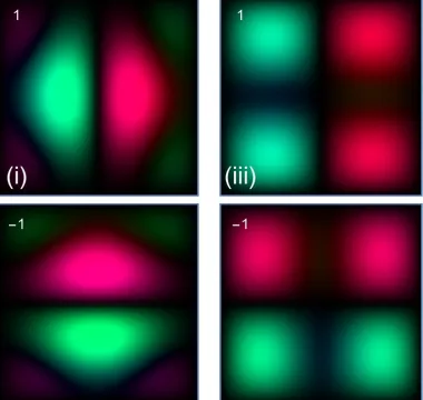
In Fig. (1) we show some of the intensity eigenmodes of the cavity for three distinct pump fields. The eigenmodes are ordered with respect to their eigenvalue which corresponds to a scaling factor of intensity at the output plane which is dependent on the modes overlap with the background field As illustrated in (i) and (iii) of the figure in cases where the background fields exhibit some n-fold rotational symmetry there exists some degenerate eigenmodes in the system. This is a result of the C4and C2 type symmetry of the pump and can be easily lifted with an additional operator in the form of a discrete rotation. Depending on the choice of rotation i.e left or right, the eigenvalues can be classified as even or odd withλ=±1 - this is shown in Fig. (2). Given the system is oscillatory the eigenmode with the largest overlap with the background will only have the highest intensity at periodic intervals. This periodicity is determined by the overlap integral, gjk = χ

R

B₁∗f₂∗_,jf3,k dr,

where the fieldsfτ are the intensity eigenmodes. This overlap integral determines both the interaction between

Figure 1: F3 components for first five intensity eigenmodes for (i) TM11, (ii) TM21 and (iii) TM22 background fields shown on the left of each panel.

Figure 2: F3 components of eigenmodes for the degenerate subspaces shown in Fig. (1)(i) on the left and Fig. (1)(iii) on the right.

3.2 Rectangular Vortex Modes

In a similar way to the transformation between Hermite-Gaussian and Laguerre-Gaussian beams8 _{we can use}

a superposition of the rectangular waveguide modes to form singular beam profiles. We denote these beams rectangular vortex modes and characterise them by the amount of ‘twist’ in the beam given by the vortex charge, l. We also adopt the convention of Laguerre-Gaussian beams and denote the radial index as p. We write the vortex modes, VTMlp as,

VTMlp=

X

where the coefficients linking the VTMlp modes the TMnm modes take the values,

cnm_lp =







i(m−1)_a N+l 2 ,

N−l 2 , m

: 2p+|l|=n+m

0 : 2p+|l| 6=n+m

where

a(n0, m0, m) =

r

(n0_+m0_{−(m−1))!(m−1)!}

2n0_+m0

n0_!m0_!

1 (m−1)!

dm0

dtm0[(1−t)

m0_{(1 +t)}n0_]|t

=0. (15)

Assuming the basis Eq. (11) is truncated with respect to some maximum mode order, N, the vortex basis can be written in full as,

flp(x, y) =Afnm(x, y). (16)

In this basis the matrices ωτ and g can be found directly from their integral form or be written in terms

of Eqs. (12) and (13) using the transformation matrix, A. Assuming the basis given by Eq. (11) is truncated with respect to some mode maximum order N, withn+m=N, this vortex basis probes the same Hilbert sub-space. However, in this representation we must consider both the field profile and the vortex charge (lb) of the

background field. In this case we consider a simplified background field of the formeilbφ_{. Due to the interaction}

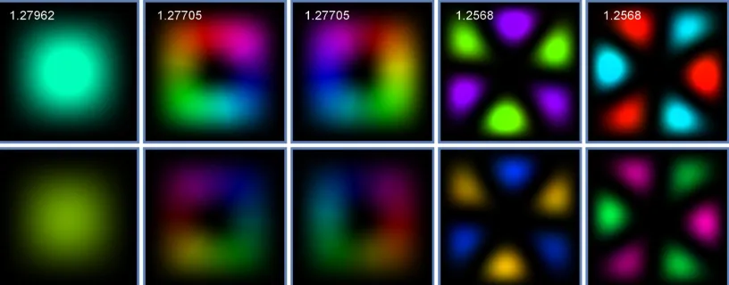
terms in Eqs. (5) to conserve the vortex charge during propagating we have the selection rule,lb=l3−l2. This is illustrated in the eigenmodes shown in Fig. (3) and (4). Note, as we are considering a thin slice of material the transfer of energy toF3 field is small and so those components of the mode are of lower intensity than the

F2 components.

Figure 3: Intensity eigenmodes for vortex background fields (not shown) of the formeilφ withlb = 0. The fields

F2 are shown above with the eigenvalue in the top left corner and the corresponding fields F3 are displayed directly below. Complex fields are represented by the false colour map with Hue showing intensity and colour showing phase.

As seen previously there exists some degeneracy due to the interaction with the complex background field. We attribute this to the angular momentum of the eigenmodes which the intensity operator can not generate. Motivated by this notion we can write the general transformations that will probe the angular momentum and commutes with the Hamiltonian, i.e Eq. (2) and (3). We find the operators,

L0_i→i(x∂y−y∂x+a) (17)

Figure 4: Intensity eigenmodes for vortex background field (not shown) of the formeilφ _{with l}

b = 1. The fields

F2 are shown above with the eigenvalue in the top left corner and the corresponding fields F3 are displayed directly below.

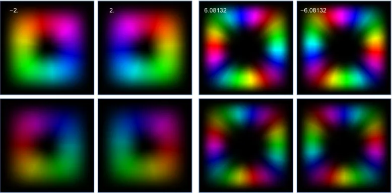
Figure 5: Degenerate eigenmodes in Fig. (3) in OAM space. The fieldsF2are shown above with the eigenvalue in the top left corner and the corresponding fieldsF3 are displayed directly below.

where a is free constant. Clearly, angular momentum itself is not a conserved quantity unless lb = 0. In

general we have to transform the operator to take into account the vortex charge of the background field. This is somewhat trivial as we cannot transform the background interaction as it exists in a Hilbert space independent of the eigenmodes. These operators can be used to lift the degeneracy of the intensity eigenmodes in Fig. (3) or indeed be used to order the eigenmodes assuming the background field is of the formeilbφ _{i.e an}

eigenfunction of the angular momentum operator, this is illustrated in Fig. (5). In this space the field components of the eigenmodes have the same vortex charge and are no longer invariant under the operationsF2→F∗3 and

4. SUMMARY AND CONCLUSION

In this paper we have extended the method of optical eigenmodes to nonlinear systems in the non-depletion approximation. We use small perturbation fields propagating in the presence of a high-intensity background interaction to define a set of orthogonal fields with interacting components in both of the available frequency channels. With these eigenmodes we highlight the influence that the complex background field has on the Hilbert space at the output plane of optical systems. In future work will look at correlations between single photons in nonlinear systems by using these eigenmodes as our orthonormal basis. Looking further we plan to extend this work to a full nonlinear theory that goes beyond the limits of the non-depleting pump approximation and expand the tools available in nonlinear sciences.

REFERENCES

[1] Mazilu, M., Baumgartl, J., Kosmeier, S., and Dholakia, K., “Optical eigenmodes; exploiting the quadratic nature of the energy flux and of scattering interactions,”Optics Express19, 933–944 (2011).

[2] De Tommasi, E., De Luca, A. C., Lavanga, L., Dardano, P., De Stefano, M., De Stefano, L., Langella, C., Rendina, I., Dholakia, K., and Mazilu, M., “Biologically enabled sub-diffractive focusing,”Optics Express22, 27215–27227 (2014).

[3] Kosmeier, S., De Luca, A., Zolotovskaya, S., Di Falco, A., Dholakia, K., and Mazilu, M., “Coherent control of plasmonic nanoantennas using optical eigenmodes,”Scientific Reports3, 1–6 (2013).

[4] De Luca, A., Kosmeier, S., Dholakia, K., and Mazilu, M., “Optical eigenmode imaging,”Physical Review A - Atomic, Molecular, and Optical Physics84, 021803 (1–6) (2011).

[5] Kosmeier, S., Zolotovskaya, S., Chiara, A., Luca, D., Riches, A., Herrington, C. S., Dholakia, K., and Mazilu, M., “Nonredundant raman imaging using optical eigenmodes,”Optica1, 257–263 (2014).

[6] Chen, M., Dholakia, K., and Mazilu, M., “Is there an optimal basis to maximise optical information trans-fer?,”Scientific Reports 6, 1–7 (2016).

[7] Shen, Y. R., [The Principles of Nonlinear Optics], John Wiley & Sons, Hoboken, New Jersey (2003). [8] O’Neil, A. and Courtial, J., “Mode transformations in terms of the constituent hermite-gaussian or