A New Software Reliability Growth Model: Genetic Programming Based Approach

doi:10.4236/jsea.2011.48054 Published Online August 2011 (http://www.SciRP.org/journal/jsea)

A New Software Reliability Growth Model:

Genetic-Programming-Based Approach

Zainab Al-Rahamneh1, Mohammad Reyalat1, Alaa F. Sheta2, Sulieman Bani-Ahmad1, Saleh Al-Oqeili1

1

Department of Information Technology, Al-Balqa Applied University, Main Campus, Salt, Jordan; 2 Department of Computer Sci-ence, The World Islamic Sciences and Education University (WISE), Amman, Jordan.

Email: {zainab, saleh}@bau.edu.jo, [email protected], [email protected], [email protected]

Received June 26th, 2011, revised July 20th, 2011, accepted July 27th, 2011.

ABSTRACT

A variety of Software Reliability Growth Models (SRGM) have been presented in literature. These models suffer many problems when handling various types of project. The reason is; the nature of each project makes it difficult to build a model which can generalize. In this paper we propose the use of Genetic Programming (GP) as an evolutionary com-putation approach to handle the software reliability modeling problem. GP deals with one of the key issues in computer science which is called automatic programming. The goal of automatic programming is to create, in an automated way,

a computer program that enables a computer to solve problems. GP will be used to build a SRGM which can predict accumulated faults during the software testing process. We evaluate the GP developed model and compare its per-formance with other common growth models from the literature. Our experiments results show that the proposed GP model is superior compared to Yamada S-Shaped, Generalized Poisson, NHPP and Schneidewind reliability models.

Keywords: Software Reliability, Genetic Programming, Modeling, Software Faults

1. Introduction

Optimistically one would think that, once software can run correctly, it will be stay so forever. A series of trage-dies and chaos caused by software proves this idea about software to be wrong. In fact, software can have small unnoticeable errors or drifts that can cause a disaster. We give two examples, On February 25, 1991, during the Gulf War against Iraq, the chopping error that missed 0.000000095 second in precision in every 10th of a sec-ond made the Patriot missile fail to intercept a scud mis-sile [1]. Another example, On June 4, 1996, the maiden flight of the Ariane 5 launcher has ended in a failure. The failure occurred only about 40 seconds after initiation of the flight sequence, the launcher veered off its flight path, broke up and exploded [2].

One of the purposes of software engineering is to pro-duce reliable software. Software plays a critical role not only in scientific and business applications, but also in all our daily life. Although several works have been done towards the production of fault-free software, developing reliable software is one of the most difficult problems facing software industry nowadays. Developing reliable software can be costly and time consuming process. Yet more, the fact that software project managers require

accurate information about how software reliability grows in order to effectively manage their budgets and projects [3-5].

Because it is a matter of economy to produce software with reliability above a given specific level, it is neces-sary to measure and, thus, control its reliability [6]. To do this, and to provide software vendors with information about their products before they are shipped to customers, a number of software reliability models have been de-veloped in literature [7].

data and the mathematical function.

Many approaches were presented to build SRGM us-ing soft-computus-ing techniques such as neural networks and fuzzy logic. Predicting accumulated faults during the software testing process using parametric and non-pa-rametric models were explored in many articles [10-12]. In [13], author provided a strategic solution for estimat-ing software defect fix effort usestimat-ing self-organizestimat-ing neural network. Fuzzy logic and neural networks were used in software engineering project management [14,15].

In this paper we present a number of software reliabil-ity growth models which successfully used to solve the reliability modeling problem, in literature. Further, we propose a genetic programming model to identify a new software reliability growth model. We comparatively evaluate the proposed model against other common growth models. We also study the efficiency of the pro-posed model in the reliability prediction process. Our experiments show that that the proposed genetic-pro- gramming model superior compared to other models found in literature.

2. Software Reliability

The demand for software systems has recently increased very rapidly. The reliability of software systems has be-come a critical issue in software systems industry. With the 90’s of the previous century, computer software sys-tems have become the major source of reported failures in many systems [16]. Software is considered reliable if anyone can depend on it and use it in critical systems. The importance of software reliability will increase in the years to come, specifically in the fields of aerospace in-dustry, satellites, and medicine applications. The process of software reliability starts with software testing and gathering of test results, after that, the phase of building a reliability model [17].

In general, the concept of reliability can be defined as “the probability that a system will perform its intended function during a period of running time without any failure” [18]. IEEE defines software reliability as “the probability of failure-free software operations for a specified period of time in a specified environment” [16, 19]. In other words, software reliability can be viewed as the analysis of its failures, their causes and effects. Soft-ware reliability is a key characteristic of product quality. Most often, specific criteria and performance measures are placed into reliability analysis, and if the performance is below a certain level, failure occurred. Mathematically, the reliability function R(t) is the probability that a sys-tem will be successfully operating without failure in the interval from time 0 to time t,

 





R t P Tt t (1)

T: is a random variable representing the failure time or time-to-failure (i.e. the expected value of the lifetime before a failure occurs). R(t) is the probability that the system's lifetime is larger than (t), the probability that the system will survive beyond time t, or the probability that the system will fail after time t. From Equation (1), we can conclude that failure probability F(t) (unreliability function of T is:

 

 





F t  R t P Tt (2) If the time-to-failure random variable T has a density function f(t), then the reliability can be measured by the following equation

 

 

t

R t f x x





_

where f(x) represents the density function for the random variable T. Consequently, the three functions, R(t), F(t) and f(t) are closely related to one another (i.e., if any of them is known, all the others can be measured and de-termined).

3. Evolutionary Computation

Several problems in artificial intelligence field need dis-covery of a computer program that produces some de-sired output for particular inputs [20,21]. The solution for these kinds of problems can be presented as the process of searching a space of possible computer programs for a most suitable individual computer program. Evolutionary Computation (EC) algorithms are a collection of algo-rithms based on the evolution of a population toward a solution of a specific problem [21]. These algorithms can be used in many applications requiring the optimization of a certain multi-dimensional function. The population of possible solutions evolves from one generation to the next, up to arriving at a suitable and satisfactory solution to the problem. EC algorithms are search algorithms that incrementally preserve and combine desirable features of individual potential solutions in a population over an extended period of time [22]. These algorithms consist of several techniques that solve computational problems by simulating evolution with natural selection.

4. Genetic Programming

strings, such as in genetic algorithms, which encode pos-sible solutions to the problem, but they are programs which represent the candidate solutions to the problem in a form of a computer program represented as a tree structure.

GAs has several disadvantages, for example the length of the strings is static and limited, and it is often hard to describe what the characters of the string means. These problems could be overcome but a better solution intro-duces again the original question: How can computers learn to solve problems without being explicitly pro-grammed?

Different problems in machine learning and artificial intelligence can be viewed as requiring the discovery of a computer program that produces some desired output for particular inputs. The process of solving these problems becomes equivalent to searching a space of possible computer programs for a highly fit individual computer program. In GP, populations of computer programs are genetically bred using the Darwinian principle of sur-vival of the fittest and using a genetic crossover (sexual recombination) operator appropriate for genetically mat-ing computer programs [23]. Genetic programmmat-ing tech-niques deal with one of the key issues in computer sci-ence which is called automatic programming. The goal of automatic programming is to create, in an automated way, a computer program that enables a computer to solve a problem, or in other words as in [24], the goal of auto-matic programming can be understood after answering the question: How can computers be made to do what needs to be done, without being told exactly how to do it.

5. Software Reliability Growth Models

Software reliability models are statistical models, which can be used to make predictions about software system's failure rate, given the failure history of the system. The models make assumptions about the fault discovery and removal process. These assumptions describe the form of the model and the meaning of the model’s parameters [17].

The models can be classified according to the nature of the failure process as Times between Failures models. The time between (j-1)st and jth failures follows a dis-tribution with parameters depending on the number of failures remaining in the program during this interval and it is expected that these intervals will increase as faults are removed. But, this may not be true for each pair of successive failure times, because failure times are ran-dom variables and observed values are subject to statis-tical changes. Next we describe a number of software reliability models that can be found in literature.

5.1. The Exponential Model

The most widely used software reliability growth model is the exponential model. It is originally proposed by Jelinski and Moranda [25], and then many variations have appeared. The original Jelinski and Moranda expo-nential model made use of the elapsed wall clock time when a failure was encountered. An important modifica-tion was made by Musa, who refined the model in terms of CPU execution time allowing for more accurate pre-dictions. Latter, Goel and Okumoto worked to generalize the model, allowing the initial number of errors in a pro-gram to be random rather than fixed, and permitting er-rors to be independent. This model remains popular and widely used although it has been shown [26] that the exponential model is not generally the most accurate software reliability growth model.

5.2. The Logarithmic Model

The logarithmic model was originally proposed by Musa and Okumoto [27]. The important difference between this model and the exponential model is that the loga-rithmic model assumes that failure intensity will decrease exponentially with the expected number of failures ob-served, while the exponential model assumes an equal reduction in failure intensity with each fault observed and corrected.

5.3. Other Models

Jelinski-Moranda (J-M) model [25] has a simple struc-ture and assumptions. This Musa’s basic model was de-veloped in 1975 [27]. It was the first one to explicitly require that the time measurements are in actual CPU time (not calendar time). This model has similar assump-tions to those of J-M model [3].

6. Proposed GP Model

Measuring the quality of software products has become one of the basic challenges in software projects. A soft-ware product can be released only after some specific reliability criterion has been satisfied. It is necessary to use some heuristics to estimate the needed testing time so that available resources can be efficiently allocated. Software reliability growth models are used to describe and predict the fault population contained within the software product.

A number of software reliability growth models are now available. It is widely known that none of these models performs well in all situations [26,28-30]. For this reason recent work has focused on developing mod-els which can be more accurate, rather than trying to find a model which works in all cases.

suggested, and some appear to be better than others. But, models that are good overall are not always the best choice for a particular data set [3] and it is not possible to know which model to use a priori [6]. Even when an appropriate model is used, the predictions made by a model may still be less accurate than desired. So, recent researches are trying to develop models that are appro-priate and efficient for a particular data set. In order to develop a software reliability growth model for particular data sets, the following steps have been performed.

GP Tuning Parameters

In order to develop new software reliability growth mod-el using genetic programming techniques, it is very nec-essary to adopt, recalibrate and adjust the genetic opera-tors and parameters. We have used “lilgp” Programming package [5,31] to accomplish the implementation. In this part, several adjustments have been made for the genetic operators and parameters. The adjusted operations and parameters are:

The set of used functions

“Plus”, “minus” and “multiply” are the functions used as a basis to develop a new model.

The “depth nodes” parameter

“depth nodes” parameter takes one of two values. If is set to 1, this means that values of other parameters (i.e.

initial maximum level, initial dynamic level, real maxi-mum level) will point to the maximaxi-mum depth of the tree. If “depth nodes” is set to 2, values of parameters will point to the size of the tree (i.e. number of nodes). Con-trol over maximum depth of the tree and size of the tree at the same time is allowed.

Initial maximum level, initial dynamic level and real maximum level of the tree

In order to avoid “bloat”, a phenomenon consisting of an excessive code growth without the corresponding im-provement in fitness, Trees in genetic programming may be subject to a set of restrictions on size, by setting ap-propriate parameters. The standard way of avoiding bloat is by setting a maximum depth on trees being evolved. Consequently, whenever a genetic operator produces a tree that breaks this limit, one of its parents enters the new population instead [21].

The processing for the initial maximum level, initial dynamic level and real maximum level can be performed in the following schema. For each new tree produced by a genetic operator, there are three possibilities:

 The new tree does not exceed the “dynamic maxi-mum level”. In this case, the new tree will be ac-cepted because no constraints have been violated.

 The new tree is larger than the “dynamic maximum level”, but does not exceed the strict “real maximum level”. In this case, the fitness of the tree is measured.

If the tree is better than the best tree found so far, “the dynamic maximum level” is increased and the new tree is accepted into the population; otherwise, the new tree is rejected and one of its parents enters the population instead.

 The new tree is larger than the strict “real maximum level”. In this case, the tree is rejected and one of its parents enters the population instead.

 The “dynamic maximum level” technique is a recent technique that has shown to effectively control bloat [31].

Determining the population size

The population size is set to 2000. We have designed too many experiments to explore the efficient value of the population size. When we explore values larger than 2000, this caused some overhead on the system without increasing the fitness of the produced model. Taking values less than 2000 may not produce the optimal solu-tion. Choosing the value 2000 in our work is experimen-tal result.

Determining the maximum number of generations

The maximum number of generations is set to 100. The experimental results show that choosing the value 100 decreased the overhead on the system and led to the most-likely optimal solution.

Determining the crossover and mutation rates

The crossover rate is set to 0.8, and the mutation rate is set to 0.01.

Determining the fitness measure

Normalized RMSE (Root Mean Square Error) is se-lected as a fitness measure. The RMSE statistic is also known as the fit standard error and the standard error of the regression. An RMSE value closer to zero indicates a better fit. The equation that responsible for calculating the normalized RMSE is





1

1 1 n

i

i i NRMSE

n n 

y z







where

n: is the number of data points.

yi: is the ithpoint of the observed data (original data).

zi: is the ithpoint of the fitted data (model prediction).

7. Experimental Results

measurement tool that can perform different functions as making reliability estimates, determining the applicabil-ity of a particular model to a set of failure data, display-ing the results given by the software reliability models graphically, and allowing users to define several types of combination models. CASER was used to develop the results for four reliability growth model for the sake of comparison with the GP model. The experimental data sets were collected from [32].

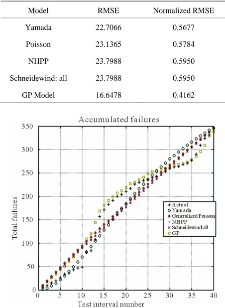
Our objective is to study the relation between test in-terval number and accumulated number of failures. In order to evaluate the ability of the proposed models to predict the behavior of the software after releasing it to the market, a data set represents 60% of the studied data were used in the training phase whereas the rest of the data were used in the testing phase. The experimental results (Table 1) showed that the proposed model achieved a good level of estimation for the reliability of the software product after releasing it in the future.

The results in the Table 1 show that the proposed GP model has achieved the best performance over all of the studied models.

Table 1. RMSE values for the studied software reliability models.

Model RMSE Normalized RMSE

Yamada 22.7066 0.5677

Poisson 23.1365 0.5784

NHPP 23.7988 0.5950

Schneidewind: all 23.7988 0.5950

GP Model 16.6478 0.4162

Figure 1. Accumulated failures for CASRE models and GP model.

Figure 2. The convergence process for the proposed model.

Figure 1 shows the proposed GP-based approach was the closest to actual curve of the experimental data. Figure 2

displays the convergence curve for the proposed model. This figure shows the relation between number of gen-erations and the fitness value that represents the normal-ized RMSE. Figure 2 shows that the GP model is capa-ble to significantly converge within around 80 genera-tions.

8. Conclusions

In this paper, we development a new software reliability growth model based genetic programming. In our pro-posed model, we adopted recalibrated and adjusted GP operators and parameters to speed up the convergence process. The GP model was compared with well known model in the. The results show that the proposed GP model gained the best performance with the adopted data sets provided in [32].

REFERENCES

[1] D. N. Arnold, “Two Disasters Caused by Computer Arithmetic Errors,” 2010.

http://www.ima.umn.edu/~arnold/455.f96/disasters.html. Viewed in December 2010.

[2] J. L. Lions, “ARIANE 5 Flight 501 Failure—Report by the Inquiry Board,” December 2010.

http://www.di.unito.it/~damiani/ariane5rep.html.

[3] G. Junhong, Y. Xiaozong and L. Hongwei, “Software Reliability Nonlinear Modeling and Its Fuzzy Evalua-tion,” 4th WSEAS International Conference, 2005.

[4] A. Yadav and R. A. Khan, “Software Reliability,” Pro-ceedings of INDIACom-2009, 2009.

[6] V. Almering, M. Genuchten, G. Cloudt and P. J. M. Son-nemans, “Using Software Reliability Growth Models in Practice,” IEEE Software, Vol. 24, No. 6, November 2007, pp. 82-88.

[7] H. Okamura and T. Dohi, “Building Phase-Type Software Reliability Models,” 17th International Symposium on Software Reliability Engineering, 2006 (ISSRE’06), 7-10 November 2006, pp. 289-298.

[8] J. D. Pfefferman and B. Cernuschi-Frias, “A Nonpara-metric Nonstationary Procedure for Failure Prediction,” IEEE Transactions on Reliability, Vol. 51, No. 4, De-cember 2002, pp. 434-442. doi:10.1109/TR.2002.804733

[9] P. B. Lakey and A. M. Neufelder, “System Software Re-liability Assurance Notebook,” P. Lakey Boeing Corpora-tion, 1997.

http://www.cs.colostate.edu/~cs530/rh/master01.pdf.

[10] S. Aljahdali, D. Rine and A. Sheta, “Prediction of Soft-ware Reliability: A Comparison between Regression and Neural Network Nonparametric Models,” ACS/IEEE In-ternational Conference on Computer Systems and Appli-cations (AICCSA 2001), Beirut, 2001, pp. 470-473.

doi:10.1109/AICCSA.2001.934046

[11] S. Aljahdali, A. Sheta and D. Rine, “Predicting Accumu-lated Faults in Software Testing Process Using Radial Basis Function Network Models,” 17th International Conference on Computers and Their Applications (CATA), Special Session on Intelligent Software Reliabil-ity, San Francisco, 2002.

[12] A. Sheta, “Reliability Growth Modeling for Software Fault Detection Using Particle Swarm Optimization,” 2006 IEEE Congress on Evolutionary Computation, Sheraton, Vancouver Wall Centre, Vancouver, 16-21 July 2006, pp. 10428-10435.

[13] H. Zeng and D. Rine, “A Neural Network Approach for Software Defects Fix Effort Estimation,” Proceedings of the Eighth IASTED International Conference Software Engineering and Applications, 2004, pp. 513-517.

[14] A. C. Hodgkinson and P. W. Garratt, “A Neurofuzzy Cost Estimator,” Proceedings of the Third Conference on Software Engineering and Applications, 1999, pp. 401- 406.

[15] S. Kumar, B. A. Krishna and P. S. Satsangi, “Fuzzy Sys-tems and Neural Networks in Software Engineering Pro-ject Management,” Journal of Applied Intelligence, Vol. 4, 1994, pp. 31-52. doi:10.1007/BF00872054

[16] S. R. Dalal, M. R. Lyu and C. L. Mallows, “Software Reliability,” Bellcore, Lucent Technologies, AT&T Re-search, 1998.

[17] C. A. Asad, M. I. Ullah and M. Jaffar-Ur Rehman, “An Approach for Software Reliability Model Selection,” 28th Annual International Computer Software and Applica-tions Conference (COMPSAC’04), 2004, pp. 534-539.

[18] J. D. Musa, “Software Reliability Engineering: More Reliable Software, Faster Development and Testing,” McGraw-Hill, New York, 1998.

[19] IEEE, “Standard Glossary of Software Engineering Ter-minology,” STD-729-1991, ANSI/IEEE, 1991.

[20] A. Robinson, J. Davila and M. Feinstein, “Genetic Pro-gramming: Theory, Implementation, and the Evolution of Unconstrained Solutions,” Hampshire College, 2001.

[21] J. R. Koza, “Genetic Programming: On the Programming of Computers by Means of Natural Selection,” 6th Edi-tion, Massachusetts Institute of Technology, The MIT Press, Cambridge, 1998.

[22] J. A. Foster, “Evolutionary Computation,” Technical Report, Department of Computer Science. Digital Genet-ics Workgroup, Lab for Applied Logic, The University of Idaho, February 1998.

http://citeseerx.ist.psu.edu/viewdoc/download;jsessioid=B B08A0A2336B38D5A82F8F8121729500?doi=10.1.1.49. 9833&rep=rep1&type=pdf.

[23] J. R. Koza, “Genetic Programming: A Paradigm for Ge-netically Breeding Populations of Computer Programs to Solve Problems,” Technical Report, Stanford University, Stanford, 1990.

http://portal.acm.org/citation.cfm?id=892491.

[24] A. L. Samuel, “Some Studies in Machine Learning Using the Game of Checkers,” MIT Press, Cambridge, 1995, pp. 71-105.

[25] Z. Jelinski and P. B. Moranda, “Software Reliability Re-search,” In: W. Freiberger, Ed., Statistical Computer Per-formance Evaluation, Academic Press, New York, 1972, pp. 465-484.

[26] Y. K. Malaiya, N. Karunanithi and P. Verma, “Predict-ability of Software-Reli“Predict-ability Models,” IEEE Transac-tions on Reliability, Vol. 41, No. 4, December 1992, pp. 539-546. doi:10.1109/24.249581

[27] J. D. Musa, “A Theory of Software Reliability and Its Application,” IEEE Transactions on Software Engineer-ing, Vol. 1, No. 3, 1975, pp. 312-327.

[28] P. A. Killer and D. R. Miller, “On the Use and Perform-ance of Software Reliability Growth Models,” Reliability Engineering and System Safety, Vol. 32, No. 1-2, 1991, pp. 95-117. doi:10.1016/0951-8320(91)90049-D

[29] T. M. Khoshgoftaar and T. G. Woodcock, “Software Reliability Model Selection: A Cast Study,” Proceedings of International Symposium on Software Reliability En-gineering, Austin, 17-18 May 1991, pp. 183-191.

[30] G. J. Knaf and J. Sacks, “Software Reliability Model Selection,” Proceedings of Computer Software and Ap-plication Conference, September 1991, pp. 597-601.

[31] D. Zongker and B. Punch, “lil-gp 1.01 User’s Manual,” Bill Rand Michigan State University, March 1996.