A Tabular Method for Dynamic Oracles in Transition-Based Parsing
Yoav Goldberg Department of Computer Science Bar Ilan University, Israel [email protected]
Francesco Sartorio Department of Information Engineering University of Padua, Italy [email protected]
Giorgio Satta Department of Information Engineering University of Padua, Italy [email protected]
Abstract
We develop parsing oracles for two trans-ition-based dependency parsers, including the arc-standard parser, solving a problem that was left open in (Goldberg and Nivre, 2013). We experimentally show that using these or-acles during training yields superior parsing accuracies on many languages.
1 Introduction
Greedy transition-based dependency parsers (Nivre, 2008) incrementally process an input sentence from left to right. These parsers are very fast and provide competitive parsing accuracies (Nivre et al., 2007). However, greedy transition-based parsers still fall behind search-based parsers (Zhang and Clark, 2008; Huang and Sagae, 2010) with respect to accuracy.
The training of transition-based parsers relies on a component called the parsingoracle, which maps parser configurations to optimal transitions with re-spect to a gold tree. A discriminative model is then trained to simulate the oracle’s behavior. A parsing oracle is deterministic if it returns a single canon-ical transition. Furthermore, an oracle is partial if it is defined only for configurations that can reach the gold tree, that is, configurations representing pars-ing histories with no mistake. Oracles that are both deterministic and partial are calledstatic. Tradition-ally, only static oracles have been exploited in train-ing of transition-based parsers.
Recently, Goldberg and Nivre (2012; 2013) showed that the accuracy of greedy parsers can be substantially improved without affecting their pars-ing speed. This improvement relies on the intro-duction of novel oracles that are nondeterministic
and complete. An oracle is nondeterministic if it re-turns the set of all transitions that are optimal with respect to the gold tree, and it is complete if it is well-defined and correct for every configuration that is reachable by the parser. Oracles that are both non-deterministic and complete are calleddynamic.
Goldberg and Nivre (2013) develop dynamic or-acles for several transition-based parsers. The con-struction of these oracles is based on a property of transition-based parsers that they call arc decompos-ition. They also prove that the popular arc-standard system (Nivre, 2004) is not arc-decomposable, and they leave as an open research question the construc-tion of a dynamic oracle for the arc-standard system. In this article, we develop one such oracle (§4) and prove its correctness (§5).
An extension to the arc-standard parser was presented by Sartorio et al. (2013), which relaxes the bottom-up construction order and allows mixing of bottom-up and top-down strategies. This parser, called here the LR-spine parser, achieves state-of-the-art results for greedy parsing. Like the arc-stand-ard system, the LR-spine parser is not arc-decom-posable, and a dynamic oracle for this system was not known. We extend our oracle for the arc-stand-ard system to work for the LR-spine system as well (§6).
The dynamic oracles developed by Goldberg and Nivre (2013) for arc-decomposable systems are based on local properties of computations. In con-trast, our novel dynamic oracle algorithms rely on arguably more complex structural properties of com-putations, which are computed through dynamic programming. This leaves open the question of whether a machine-learning model can learn to ef-fectively simulate such complex processes: will the
benefit of training with the dynamic oracle carry over to the arc-standard and LR-spine systems? We show experimentally that this is indeed the case (§8),
and that using the training-with-exploration method of (Goldberg and Nivre, 2013) with our dynamic programming based oracles yields superior parsing accuracies on many languages.
2 Arc-Standard Parser
In this section we introduce the arc-standard parser of Nivre (2004), which is the model that we use in this article. To keep the notation at a simple level, we only discuss the unlabeled version of the parser; however, a labeled extension is used in §8 for our
experiments.
2.1 Preliminaries and Notation
The set of non-negative integers is denoted as N0. For i, j ∈ N0 withi ≤ j, we write[i, j]to denote the set{i, i+ 1, . . . , j}. Wheni > j,[i, j]denotes
the empty set.
We represent an input sentence as a string w =
w0· · ·wn, n ∈ N0, where token w0 is a special root symbol, and each wi with i ∈ [1, n]is a
lex-ical token. For i, j ∈ [0, n]with i ≤ j, we write w[i, j]to denote the substringwiwi+1· · ·wjofw.
We write i → j to denote a grammatical
de-pendencyof some unspecified type between lexical tokenswiandwj, wherewiis the head andwj is the
dependent. Adependency treeforwis a directed,
ordered treet = (Vw, A), such that Vw = [0, n]is
the set of nodes,A⊆Vw×Vwis the set of arcs, and
node0is the root. Arc(i, j)encodes a dependency
i → j, and we will often use the latter notation to
denote arcs.
2.2 Transition-Based Dependency Parsing We assume the reader is familiar with the formal framework of transition-based dependency parsing originally introduced by Nivre (2003); see Nivre (2008) for an introduction. We only summarize here our notation.
Transition-based dependency parsers use a stack data structure, where each stack element is associ-ated with a tree spanning (generating) some sub-string of the inputw. The parser processes the
in-put string incrementally, from left to right, applying at each step a transition that updates the stack and/or
consumes one token from the input. Transitions may also construct new dependencies, which are added to the current configuration of the parser.
We represent the stack data structure as an ordered sequence σ = [σd, . . . , σ1], d ∈ N0, of nodes σi ∈ Vw, with the topmost element placed
at the right. Whend= 0, we have the empty stack
σ = []. Sometimes we use the vertical bar to denote
the append operator forσ, and writeσ = σ0|σ1 to indicate thatσ1is the topmost element ofσ.
The parser also uses abufferto store the portion of the input string still to be processed. We represent the buffer as an ordered sequenceβ = [i, . . . , n]of
nodes from Vw, withithe first element of the
buf-fer. In this wayβalways encodes a (non-necessarily
proper) suffix ofw. We denote the empty buffer as β = []. Sometimes we use the vertical bar to denote
the append operator forβ, and writeβ =i|β0 to
in-dicate thatiis the first token ofβ; consequently, we
haveβ0 = [i+ 1, . . . , n].
When processing w, the parser reaches several
states, technically called configurations. A config-uration of the parser relative to w is a triple c = (σ, β, A), where σ andβ are a stack and a buffer,
respectively, andA⊆Vw×Vw is a set of arcs. The
initialconfiguration forw is([],[0, . . . , n],∅). For
the purpose of this article, a configuration is final if it has the form ([0],[], A), and in a final
config-uration arc setA always defines a dependency tree
forw.
The core of a transition-based parser is the set of its transitions, which are specific to each family of parsers. A transition is a binary relation defined over the set of configurations of the parser. We use symbol`to denote the union of all transition rela-tions of a parser.
Acomputationof the parser onwis a sequence c0, . . . , cm,m ∈ N0, of configurations (defined rel-ative tow) such thatci−1 ` ci for eachi ∈ [1, m].
We also use the reflexive and transitive closure rela-tion`∗to represent computations. A computation is calledcompletewheneverc0 is initial andcm is
fi-nal. In this way, a complete computation is uniquely associated with a dependency tree forw.
2.3 Arc-Standard Parser
(σ, i|β, A)`sh(σ|i, β, A)
(σ|i|j, β, A)`la(σ|j, β, A∪ {j→i}) (σ|i|j, β, A)`ra(σ|i, β, A∪ {i→j})
Figure 1: Transitions in the arc-standard model.
• Shift (sh) removes the first node in the buffer and pushes it into the stack;
• Left-Arc (la) creates a new arc with the topmost node on the stack as the head and the second-topmost node as the dependent, and removes the second-topmost node from the stack;
• Right-Arc (ra) is symmetric tolain that it
cre-ates an arc with the second-topmost node as the head and the topmost node as the dependent, and removes the topmost node.
Notation We sometimes use the functional nota-tion for a transinota-tion τ ∈ {sh,la,ra}, and write
τ(c) = c0 in place ofc `τ c0. Naturally,shapplies
only when the buffer is not empty, andla,rarequire
two elements on the stack. We denote by valid(c)
the set of valid transitions in a given configuration. 2.4 Arc Decomposition
Goldberg and Nivre (2013) show how to derive dy-namic oracles for any transition-based parser which has the arc decomposition property, defined below. They also show that the arc-standard parser is not arc-decomposable.
For a configurationc, we writeActo denote the
associated set of arcs. A transition-based parser is arc-decomposableif, for every configurationcand
for every set of arcsAthat can be extended to a
pro-jective tree, we have
∀(i→j)∈A,∃c0[c`∗c0∧(i→j)∈Ac0] ⇒ ∃c00[c`∗c00∧A⊆Ac00].
In words, if each arc inA is individually derivable
fromc, then the setAin its entirety can be derived from c as well. The arc decomposition property
is useful for deriving dynamic oracles because it is relatively easy to investigate derivability for single arcs and then, using this property, draw conclusions about the number of gold-arcs that are simultan-eously derivable from the given configuration.
Unfortunately, the standard parser is not arc-decomposable. To see why, consider a configura-tion with stack σ = [i, j, k]. Consider also arc set
A = {(i, j),(i, k)}. The arc (i, j) can be derived through the transition sequence ra, ra, and the arc
(i, k) can be derived through the alternative
trans-ition sequencela,ra. Yet, it is easy to see that a con-figuration containing both arcs cannot be reached.
As we cannot rely on the arc decomposition prop-erty, in order to derive a dynamic oracle for the arc-standard model we need to develop more sophistic-ated techniques which take into account the interac-tion among the applied transiinterac-tions.
3 Configuration Loss and Dynamic Oracles We aim to derive a dynamic oracle for the arc-stand-ard (and related) system. This is a function that takes a configurationcand a gold treetGand returns a set
of transitions that are “optimal” for c with respect
totG. As already mentioned in the introduction, a
dynamic oracle can be used to improve training of greedy transition-based parsers. In this section we provide a formal definition for a dynamic oracle.
Let t1 and t2 be two dependency trees over the same stringw, with arc setsA1andA2, respectively. We define thelossoft1with respect tot2 as
L(t1, t2) =|A1\A2| . (1)
Note that L(t1, t2) = L(t2, t1), since |A1| = |A2|. Furthermore L(t1, t2) = 0 if and only ift1 andt2 are the same tree.
Letc be a configuration of our parser relative to input stringw. We writeD(c) to denote the set of
all dependency trees that can be obtained in a com-putation of the formc`∗ cf, wherecf is some final
configuration. We extend the loss function in (1) to configurations by letting
L(c, t2) = min t1∈D(c) L
(t1, t2). (2)
Assume some reference (desired) dependency treetGforw, which we call thegoldtree. Quantity L(c, tG) can be used to compute a dynamic oracle
relating a parser configurationcto a set of optimal
actions by setting
oracle(c, tG) =
We therefore need to develop an algorithm for com-puting (2). We will do this first for the arc-standard parser, and then for an extension of this model. Notation We also apply the loss functionL(t, tG)
in (1) when t is a dependency tree for a substring
of w. In this case the nodes of t are a subset of
the nodes of tG, and L(t, tG) provides a count of
the nodes oftthat are assigned a wrong head node,
whentGis considered as the reference tree.
4 Main Algorithm
Throughout this section we assume an arc-standard parser. Our algorithm takes as input a projective gold treetGand a configurationc= (σL, β, A). We
callσLtheleft stack, in contrast with a right stack
whose construction is specified below. 4.1 Basic Idea
The algorithm consists of two steps. Informally, in the first step we compute the largest subtrees, called here tree fragments, of the gold tree tG that have
their span entirely included in the buffer β. The
root nodes of these tree fragments are then arranged into a stack data structure, according to the order in which they appear inβand with the leftmost root in β being the topmost element of the stack. We call
this structure the right stackσR. Intuitively,σRcan
be viewed as the result of pre-computing β by
ap-plying all sequences of transitions that matchtGand
that can be performed independently of the stack in the input configurationc, that is,σL.
In the second step of the algorithm we use dy-namic programming techniques to simulate all com-putations of the arc-standard parser starting in a con-figuration with stackσLand with a buffer consisting
ofσR, with the topmost token ofσRbeing the first
token of the buffer. As we will see later, the search space defined by these computations includes the de-pendency trees forwthat are reachable from the
in-put configurationcand that have minimum loss. We then perform a Viterbi search to pick up such value. The second step is very similar to standard imple-mentations of the CKY parser for context-free gram-mars (Hopcroft and Ullman, 1979), running on an input string obtained as the concatenation ofσLand σR. The main difference is that we restrict ourselves
to parse only those constituents inσLσR that
dom-inate the topmost element ofσL (the rightmost
ele-ment, ifσLis viewed as a string). In this way, we
ac-count for the additional constraint that we visit only those configurations of the arc-standard parser that can be reached from the input configurationc. For instance, this excludes the reduction of two nodes in
σL that are not at the two topmost positions. This
would also exclude the reduction of two nodes in
σR: this is correct, since the associated tree
ments have been chosen as the largest such frag-ments inβ.
The above intuitive explanation will be made mathematically precise in §5, where the notion of
linear dependency tree is introduced. 4.2 Construction of the Right Stack
In the first step we processβ and construct a stack σR, which we call theright stackassociated withc
andtG. Each node ofσRis the root of a treetwhich
satisfies the following properties
• tis a tree fragment of the gold treetG having
span entirely included in the bufferβ;
• tisbottom-up completefortG, meaning that
for each nodeioftdifferent fromt’s root, the dependents ofiintGcannot be inσL;
• tismaximalfortG, meaning that every
super-tree oftintGviolates the above conditions.
The stackσRis incrementally constructed by
pro-cessigβfrom left to right. Each nodeiis copied into σRif it satisfies any of the following conditions
• the parent node ofiintGis not inβ;
• some dependent of i in tG is in σL or has
already been inserted inσR.
It is not difficult to see that the nodes inσRare the
roots of tree fragments oftGthat satisfy the
condi-tion of bottom-up completeness and the condicondi-tion of maximality defined above.
4.3 Computation of Configuration Loss
We start with some notation. Let `L = |σL| and `R = |σR|. We write σL[i]to denote thei-th
ele-ment ofσL andt(σL[i]) to denote the
correspond-ing tree fragment;σR[i]andt(σR[i])have a similar
Algorithm 1Computation of the loss function for the arc-standard parser 1: T[1,1](σL[1])← L(t(σL[1]), tG)
2: ford←1to`L+`R−1do . dis the index of a sub-anti-diagonal
3: forj←max{1, d−`L+ 1}tomin{d, `R}do . jis the column index
4: i←d−j+ 1 . iis the row index
5: ifi < `Lthen .expand to the left
6: for eachh∈∆i,jdo
7: T[i+ 1, j](h)←min{T[i+ 1, j](h), T[i, j](h) +δG(h→σL[i+ 1])}
8: T[i+ 1, j](σL[i+ 1])←min{T[i+ 1, j](σL[i+ 1]), T[i, j](h) +δG(σL[i+ 1]→h)}
9: ifj < `Rthen .expand to the right
10: for eachh∈∆i,jdo
11: T[i, j+ 1](h)←min{T[i, j+ 1](h), T[i, j](h) +δG(h→σR[j+ 1])}
12: T[i, j+1](σR[j+ 1])←min{T[i, j+1](σR[j+ 1]),T[i, j](h)+δG(σR[j+ 1]→h)}
13: returnT[`L, `R](0) +Pi∈[1,`L]L(t(σL[i]), tG)
Therefore the elements ofσRwhich have been
con-structed in§4.2 areσR[i],i∈[2, `R].
Algorithm 1 uses a two-dimensional array T of
size `L × `R, where each entry T[i, j] is an
as-sociation list from integers to integers. An entry
T[i, j](h) stores the minimum loss among
depend-ency trees rooted ath that can be obtained by run-ning the parser on the firstielements of stackσLand
the firstjelements of bufferσR. More precisely, let
∆i,j = {σL[k] | k∈[1, i]} ∪
{σR[k] | k∈[1, j]}. (4)
For each h ∈ ∆i,j, the entry T[i, j](h) is the
minimum loss among all dependency trees defined as above and with root h. We also assume that
T[i, j](h) is initialized to +∞ (not reported in the algorithm).
Algorithm 1 starts at the top-left corner ofT, vis-iting each individual sub-anti-diagonal of T in
as-cending order, and eventually reaching the bottom-right corner of the array. For each entryT[i, j], the
left expansion is considered (lines 5 to 8) by com-bining with tree fragmentσL[i+ 1], through a left
or a right arc reduction. This results in the update ofT[i+ 1, j](h), for eachh ∈ ∆i+1,j, whenever a
smaller value of the loss is achieved for a tree with root h. The Kronecker-like function used at line 8
provides the contribution of each single arc to the loss of the current tree. Denoting withAGthe set of
arcs oftG, such a function is defined as
δG(i→j) =
0, if(i→j)∈AG;
1, otherwise. (5)
A symmetrical process is implemented for the right expansion of T[i, j] through tree fragment
σR[j+ 1](lines 9 to 12).
As we will see in the next section, quantity
T[`L, `R](0)is the minimal loss of a tree composed
only by arcs that connect nodes inσLandσR. By
summing the loss of all tree fragments t(σL[i]) to
the loss in T[`L, `R](0), at line 13, we obtain the
desired result, since the loss of each tree fragment
t(σR[j])is zero.
5 Formal Properties
Throughout this section we let w, tG, σL, σR and c= (σL, β, A)be defined as in§4, but we no longer assume thatσL[1] =σR[1]. To simplify the
present-ation, we sometimes identify the tokens in w with
the associated nodes in a dependency tree forw.
5.1 Linear Trees
Algorithm 1 explores all dependency trees that can be reached by an arc-standard parser from configur-ationc, under the condition that (i) the nodes in the
buffer β are pre-computed into tree fragments and
collapsed into their root nodes in the right stackσR,
and (ii) nodes in σR cannot be combined together
char-j4
i6 i5 i3 j5
i4 i1 j3
[image:6.612.107.268.51.173.2]i2 j1 j2 σR σL
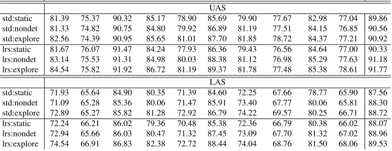
Figure 2: A possible linear tree for string pair(σL, σR),
whereσL = i6i5i4i3i2i1 and σR = j1j2j3j4j5. The spine of the tree consists of nodesj4,i3andi1.
acterized here using the notion of linear tree, to be used later in the correctness proof.
Consider two nodes σL[i] and σL[j] with j > i > 1. An arc-standard parser can construct an arc betweenσL[i]andσL[j], in any direction, only after
reaching a configuration in whichσL[i]is at the top
of the stack andσL[j]is at the second topmost
posi-tion. In such configuration we have thatσL[i]
dom-inatesσL[1]. Furthermore, consider nodesσR[i]and σR[j]withj > i ≥ 1. Since we are assuming that
tree fragmentst(σR[i])andt(σR[j])are bottom-up
complete and maximal, as defined in§4.2, we allow
the construction of an arc betweenσR[i]andσR[j],
in any direction, only after reaching a configuration in whichσR[i]dominates nodeσL[1].
The dependency trees satisfying the restrictions above are captured by the following definition. A linear treeover(σL, σR)is a projective dependency
treet for string σLσR satisfying both of the
addi-tional conditions reported below. The path fromt’s
root to nodeσL[1]is called thespineoft.
• Every node oftnot in the spine is a dependent
of some node in the spine.
• For each arci→ jintwithjin the spine, no
dependent ofican be placed in betweeniand jwithin stringσLσR.
An example of a linear tree is depicted in Figure 2. Observe that the second condition above forbids the reduction of two nodesiandj, in case none of these
dominates node σL[1]. For instance, thera
reduc-tion of nodesi3 andi2 would result in arci3 → i2 replacing arci1 →i2in Figure 2. The new depend-ency tree is not linear, because of a violation of the
second condition above. Similarly, thelareduction of nodesj3 andj4 would result in arc j4 → j3 re-placing arci3 →j3in Figure 2, again a violation of the second condition above.
Lemma 1 Any tree t ∈ D(c) can be decomposed into treest(σL[i]),i∈[1, `L], treestj,j∈[1, q]and q ≥ 1, and a linear treetl over (σL, σR,t), where σR,t=r1· · ·rqand eachrjis the root node oftj.2
PROOF(SKETCH) Trees t(σL[i]) are common to
every tree inD(c), since the arc-standard model can
not undo the arcs already built in the current con-figurationc. Similar to the construction in §4.2 of the right stackσR fromtG, we lettj,j ∈ [1, q], be
tree fragments oftthat cover only nodes associated
with the tokens in the bufferβ and that are bottom-up complete and maximal fort. These trees are
in-dexed according to their left to right order inβ.
Fi-nally,tlis implicitly defined by all arcs oftthat are
not in treest(σL[i])andtj. It is not difficult to see
thattl has a spine ending with nodeσL[1] and is a
linear tree over(σL, σR,t).
5.2 Correctness
Our proof of correctness for Algorithm 1 is based on a specific dependency treet∗forw, which we define
below. LetSL={σL[i] | i∈[1, `L]}and letDLbe
the set of nodes that are descendants of some node inSL. Similarly, letSR = {σR[i] | i ∈ [1, `R]}
and let DR be the set of descendants of nodes in SR. Note that sets SL, SR, DL andDR provide a
partition ofVw.
We choose any linear treet∗l over(σL, σR)having
root0, such thatL(t∗
l, tG) = mintL(t, tG), where tranges over all possible linear trees over (σL, σR)
with root0. Treet∗ consists of the set of nodesVw
and the set of arcs obtained as the union of the set of arcs oft∗l and the set of arcs of all treest(σL[i]), i∈[1, `L], andt(σR[j]),j ∈[1, `R].
Lemma 2 t∗ ∈ D(c). 2
PROOF(SKETCH) All tree fragmentst(σL[i])have
already been parsed and are available in the stack associated withc. Each tree fragmentt(σR[j])can
later be constructed in the computation, when a con-figurationc0is reached with the relevant segment of
wat the start of the buffer. Note also that parsing of t(σR[j])can be done in a way that does not depend
Finally, the parsing of the tree fragmentst(σR[j])
is interleaved with the construction of the arcs from the linear treet∗l, which are all of the form(i→ j)
withi, j ∈ (SL∪SR). More precisely, if(i→ j)
is an arc fromt∗l, at some point in the computation
nodesiandjwill become available at the two
top-most positions in the stack. This follows from the second condition in the definition of linear tree.
We now show that treet∗ is “optimal” within the setD(c)and with respect totG.
Lemma 3 L(t∗, tG) =L(c, tG). 2
PROOF Consider an arbitrary tree t ∈ D(c). As-sume the decomposition oftdefined in the proof of
Lemma 1, through treest(σL[i]), i ∈ [1, `L], trees tj,j∈[1, q], and linear treetlover(σL, σR,t).
Recall that an arci→ j denotes an ordered pair
(i, j). Let us consider the following partition for the
set of arcs of any dependency tree forw
A1 = (SL∪DL)×DL, A2 = (SR∪DR)×DR, A3 = (Vw×Vw)\(A1∪A2).
In what follows, we compare the lossesL(t, tG)and L(t∗, tG)by separately looking into the contribution
to such quantities due to the arcs inA1,A2 andA3. Note that the arcs of trees t(σL[i])are all in A1, the arcs of treest(σR[j])are all in A2, and the arcs of treet∗l are all in A3. Sincet andt∗ share trees t(σL[i]), when restricted to arcs in A1 quantities L(t, tG) andL(t∗, tG)are the same. When
restric-ted to arcs inA2, quantityL(t∗, tG)is zero, by
con-struction of the treest(σR[j]). ThusL(t, tG)can not
be smaller thanL(t∗, tG)for these arcs. The difficult
part is the comparison of the contribution toL(t, tG)
andL(t∗, tG)due to the arcs in A3. We deal with this below.
LetAS,Gbe the set of all arcs fromtGthat are also
in set(SL×SR)∪(SR×SL). In words,AS,G
rep-resents gold arcs connecting nodes inSLand nodes
inSR, in any direction. Within treet, these arcs can
only be found in thetl component, since nodes in SLare all placed within the spine oftl, or else at the
left of that spine.
Let us consider an arc(j → i) ∈AS,G withj ∈ SLandi∈SR, and let us assume that(j →i)is in t∗l. If tokenai does not occur inσR,t, nodeiis not
intl and(j → i) can not be an arc of t. We then
have that(j → i) contributes one unit to L(t, tG)
but does not contribute to L(t∗, tG). Similarly, let
(i → j) ∈ AS,G be such thati ∈ SR andj ∈ SL,
and assume that(i→j)is int∗l. If tokenaidoes not
occur inσR,t, arc(i→ j)can not be int. We then
have that(i → j) contributes one unit to L(t, tG)
but does not contribute toL(t∗, tG).
Intuitively, the above observations mean that the winning strategy for trees inD(c)is to move nodes from SR as much as possible into the linear tree
componenttl, in order to make it possible for these
nodes to connect to nodes inSL, in any direction. In
this case, arcs fromA3will also move into the linear tree component of a tree inD(c), as it happens in the
case oft∗. We thus conclude that, when restricted to the set of arcs inA3, quantityL(t, tG)is not
smal-ler thanL(t∗, tG), because stackσRhas at least as
many tokens corresponding to nodes inSRas stack σR,t, and becauset∗l has the minimum loss among
all the linear trees over(σL, σR).
Putting all of the above observations together, we conclude that L(t, tG) can not be smaller than L(t∗, tG). This concludes the proof, sincethas been
arbitrarily chosen inD(c).
Theorem 1 Algorithm 1 computesL(c, tG). 2
PROOF(SKETCH) Algorithm 1 implements a Vi-terbi search for trees with smallest loss among all linear trees over (σL, σR). Thus T[`L, `R](0) = L(t∗l, tG). The loss of the tree fragments t(σR[j])
is0and the loss of the tree fragmentst(σL[i])is
ad-ded at line 13 in the algorithm. Thus the algorithm returns L(t∗, tG), and the statement follows from
Lemma 2 and Lemma 3.
5.3 Computational Analysis
Following §4.2, the right stack σR can be easily
constructed in time O(n), n the length of the in-put string. We now analyze Algorithm 1. For each entry T[i, j] and for each h ∈ ∆i,j, we update T[i, j](h) a number of times bounded by a con-stant which does not depend on the input. Each up-dating can be computed in constant time as well. We thus conclude that Algorithm 1 runs in time
O(`L·`R·(`L+`R)). Quantity`L+`Ris bounded
byn, but in practice the former is significantly
Treebank, the average value of `L+`R
n is 0.29. In
terms of runtime, training is 2.3 times slower when using our oracle instead of a static oracle.
6 Extension to the LR-Spine Parser
In this section we consider the transition-based parser proposed by Sartorio et al. (2013), called here the LR-spine parser. This parser is not arc-decomposable: the same example reported in§2.4
can be used to show this fact. We therefore extend to the LR-spine parser the algorithm developed in§4. 6.1 The LR-Spine Parser
Lett be a dependency tree. The left spine of tis
an ordered sequencehi1, . . . , ipi, p ≥1, consisting of all nodes in a descending path from the root of
t taking the leftmost child node at each step. The
right spineoftis defined symmetrically. We use⊕
to denote sequence concatenation.
In the LR-spine parser each stack elementσ[i]
de-notes a partially built subtreet(σ[i])and is
represen-ted by a pair(lsi,rsi), withlsiandrsithe left and the
right spine, respectively, oft(σ[i]). We writelsi[k]
(rsi[k]) to represent thek-th element oflsi (rsi,
re-spectively). We also writer(σ[i])to denote the root
oft(σ[i]), so thatr(σ[i]) =lsi[1] =rsi[1].
Informally, the LR-spine parser uses the same transition typologies as the arc-standard parser. However, an arc(h → d) can now be created with
the head nodehchosen from any node in the spine
of the involved tree. The transition types of the LR-spine parser are defined as follows.
• Shift (sh) removes the first node from the buf-fer and pushes into the stack a new element, consisting of the left and right spines of the as-sociated tree
(σ, i|β, A)`sh(σ|(hii,hii), β, A).
• Left-Arck(lak) creates a new arch →dfrom
thek-th node in the left spine of the topmost
tree in the stack to the head of the second ele-ment in the stack. Furthermore, the two top-most stack elements are replaced by a new ele-ment associated with the resulting tree
(σ0|σ[2]|σ[1], β, A)`lak (σ0|σlak, β, A∪ {h→d}) where we have seth=ls1[k],d=r(σ[2])and σlak = (hls1[1], . . . ,ls1[k]i ⊕ls2,rs1).
• Right-Arck(rakfor short) is defined symmet-rically with respect tolak
(σ0|σ[2]|σ[1], β, A)`rak (σ0|σrak, β, A∪ {h→d})
where we have seth=rs2[k],d=r(σ[1])and σrak = (ls2,hrs2[1], . . . ,rs2[k]i ⊕rs1).
Note that, at each configuration in the LR-spine parser, there are|ls1|possiblelaktransitions, one for each choice of a node in the left spine of t(σ[1]);
similarly, there are |rs2| possible rak transitions, one for each choice of a node in the right spine of
t(σ[2]).
6.2 Configuration Loss
We only provide an informal description of the ex-tended algorithm here, since it is very similar to the algorithm in§4.
In the first phase we use the procedure of§4.2 for the construction of the right stack σR, considering
only the roots of elements in σL and ignoring the
rest of the spines. The only difference is that each elementσR[j]is now a pair of spines(lsR,j,rsR,j).
Since tree fragmentt(σR[j])is bottom-up complete
(see§4.1), we now restrict the search space in such a way that only the root noder(σR[j])can take
de-pendents. This is done by settinglsR,j = rsR,j = hr(σR[j])ifor eachj∈[1, `R]. In order to simplify
the presentation we also assumeσR[1] = σL[1], as
done in§4.3.
In the second phase we compute the loss of an in-put configuration using a two-dimensional arrayT,
defined as in §4.3. However, because of the way transitions are defined in the LR-spine parser, we now need to distinguish tree fragments not only on the basis of their roots, but also on the basis of their left and right spines. Accordingly, we define each entryT[i, j]as an association list with keys of the
form(ls,rs). More specifically,T[i, j](ls,rs) is the
minimum loss of a tree with left and right spinesls andrs, respectively, that can be obtained by running the parser on the firstielements of stackσLand the
firstjelements of bufferσR.
We follow the main idea of Algorithm 1 and ex-pand each tree inT[i, j]at its left side, by
combin-ing with tree fragmentt(σL[i+ 1]), and at its right
Tree combination deserves some more detailed dis-cussion, reported below.
We consider the combination of a tree ta from T[i, j]and treet(σL[i+ 1])by means of a left-arc
transition. All other cases are treated symmetric-ally. Let (lsa,rsa) be the spine pair of ta, so that
the loss oftais stored in T[i, j](lsa,rsa). Let also
(lsb,rsb) be the spine pair of t(σL[i+ 1]). In case
there exists a gold arc intGconnecting a node from
lsa to r(σL[i+ 1]), we choose the transition lak, k∈[1,|lsa|], that creates such arc. In case such gold
arc does not exists, we choose the transitionlakwith
the maximum possible value ofk, that is,k=|lsa|.
We therefore explore only one of the several pos-sible ways of combining these two trees by means of a left-arc transition.
We remark that the above strategy is safe. In fact, in case the gold arc exists, no other gold arc can ever involve the nodes oflsa eliminated by lak (see the
definition in§6.1), because arcs can not cross each other. In case the gold arc does not exist, our choice ofk=|lsa|guarantees that we do not eliminate any element fromlsa.
Once a transition lak is chosen, as described
above, the reduction is performed and the spine pair (ls,rs) for the resulting tree is computed from (lsa,rsa) and(lsb,rsb), as defined in §6.1. At the
same time, the loss of the resulting tree is com-puted, on the basis of the loss T[i, j](lsa,rsa), the
loss of treet(σL[i+ 1]), and a Kronecker-like
func-tion defined below. This loss is then used to update
T[i+ 1, j](ls,rs).
Lettaandtb be two trees that must be combined
in such a way that tb becomes the dependent of
some node in one of the two spines ofta. Let also pa = (lsa,rsa)andpb = (lsb,rsb)be spine pairs for taandtb, respectively. Recall thatAGis the set of
arcs oftG. The new Kronecker-like function for the
computation of the loss is defined as
δG(pa, pb) =
0, ifr(ta)< r(tb)∧
∃k[(rska→r(tb))∈AG];
0, ifr(ta)> r(tb)∧
∃k[(lska→r(tb))∈AG];
1, otherwise.
6.3 Efficiency Improvement
The algorithm in§6.2 has an exponential behaviour. To see why, consider trees inT[i, j]. These trees are
produced by the combination of trees inT[i−1, j]
with treet(σL[i]), or by the combination of trees in T[i, j−1]with treet(σR[j]). Since each
combin-ation involves either a left-arc or a right-arc trans-ition, we obtain a recursive relation that resolves into a number of trees inT[i, j]bounded by4i+j−2.
We introduce now two restrictions to the search space of our extended algorithm that result in a huge computational saving. For a spines, we writeN(s)
to denote the set of all nodes ins. We also let∆i,jbe
the set of all pairs(ls,rs) such thatT[i, j](ls,rs) 6= +∞.
• Every time a new pair (ls,rs) is created in ∆[i, j], we remove fromls all nodes different from the root that do not have gold dependents in{r(σL[k]) | k < i}, and we remove from
rsall nodes different from the root that do not have gold dependents in{r(σR[k]) | k > j}.
• A pair pa = (lsa,rsa) is removed from
∆[i, j] if there exists a pair pb = (lsb,rsb)
in ∆[i, j] with the same root node as pa and
with(lsa,rsa) 6= (lsb,rsb), such thatN(lsa)⊆ N(lsb), N(rsa) ⊆ N(rsb), andT[i, j](pa) ≥ T[i, j](pb).
The first restriction above reduces the size of a spine by eliminating a node if it is irrelevant for the com-putation of the loss of the associated tree. The second restriction eliminates a tree ta if there is a
tree tb with smaller loss than ta, such that in the
computations of the parser tb provides exactly the
same context as ta. It is not difficult to see that
the above restrictions do not affect the correctness of the algorithm, since they always leave in our search space some tree that has optimal loss.
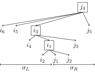
A mathematical analysis of the computational complexity of the extended algorithm is quite in-volved. In Figure 3, we plot the worst case size of T[i, j] for each value of j +i −1, computed
over all configurations visited in the training phase (see §7). We see that |T[i, j]| grows linearly with
j+i−1, leading to the same space requirements of
0 10 20 30 40 50 0
10 20 30 40 50
i+j−1
max
number
of
[image:10.612.127.244.58.192.2]elements
Figure 3: Empirical worst case size ofT[i, j] for each value of i+j −1 as measured on the Penn Treebank corpus.
Algorithm 2 Online training for greedy transition-based parsers
1: w←0
2: forkiterationsdo
3: shuffle(corpus)
4: forsentencewand gold treetGin corpusdo
5: c← INITIAL(w)
6: while notFINAL(c)do
7: τp ←argmaxτ∈valid(c)w·φ(c, τ) 8: τo ←argmaxτ∈oracle(c,tG)w·φ(c, τ) 9: ifτp6∈oracle(c, tG)then
10: w←w+φ(c, τo)−φ(c, τp)
11: τ ←
(
τp if EXPLORE τo otherwise
12: c←τ(c) returnaveraged(w)
oracle is only about 8 times slower than training with the oracle of Sartorio et al. (2013) without exploring incorrect configurations.
7 Training
We follow the training procedure suggested by Goldberg and Nivre (2013), as described in Al-gorithm 2. The alAl-gorithm performs online learning using the averaged perceptron algorithm. A weight vectorw(initialized to 0) is used to score the valid transitions in each configuration based on a feature representationφ, and the highest scoring transition
τp is predicted. If the predicted transition is not
optimal according to the oracle, the weights ware updated away from the predicted transition and
to-wards the highest scoring oracle transitionτo. The
parser then moves to the next configuration, by tak-ing either the predicted or the oracle transition. In the “error exploration” mode (EXPLOREis true), the parser follows the predicted transition, and other-wise the parser follows the oracle transition. Note that the error exploration mode requires the com-pleteness property of a dynamic oracle.
We consider three training conditions: static, in which the oracle is deterministic (returning a single canonical transition for each configuration) and no error exploration is performed;nondet, in which we use a nondeterministic partial oracle (Sartorio et al., 2013), but do not perform error exploration; and ex-plorein which we use the dynamic oracle and per-form error exploration. Thestaticsetup mirrors the way greedy parsers are traditionally trained. The nondetsetup allows the training procedure to choose which transition to take in case of spurious ambigu-ities. Theexploresetup increases the configuration space explored by the parser during training, by ex-posing the training procedure to non-optimal con-figurations that are likely to occur during parsing, together with the optimal transitions to take in these configurations. It was shown by Goldberg and Nivre (2012; 2013) that thenondetsetup outperforms the staticsetup, and that theexplore setup outperforms thenondetsetup.
8 Experimental Evaluation
Datasets Performance evaluation is carried out on CoNLL 2007 multilingual dataset, as well as on the Penn Treebank (PTB) (Marcus et al., 1993) conver-ted to Stanford basic dependencies (De Marneffe et al., 2006). For the CoNLL datasets we use gold part-of-speech tags, while for the PTB we use auto-matically assigned tags. As usual, the PTB parser is trained on sections 2-21 and tested on section 23.
parser:train Arabic Basque Catalan Chinese Czech English Greek Hungarian Italian Turkish PTB UAS
std:static 81.39 75.37 90.32 85.17 78.90 85.69 79.90 77.67 82.98 77.04 89.86 std:nondet 81.33 74.82 90.75 84.80 79.92 86.89 81.19 77.51 84.15 76.85 90.56 std:explore 82.56 74.39 90.95 85.65 81.01 87.70 81.85 78.72 84.37 77.21 90.92 lrs:static 81.67 76.07 91.47 84.24 77.93 86.36 79.43 76.56 84.64 77.00 90.33 lrs:nondet 83.14 75.53 91.31 84.98 80.03 88.38 81.12 76.98 85.29 77.63 91.18 lrs:explore 84.54 75.82 91.92 86.72 81.19 89.37 81.78 77.48 85.38 78.61 91.77
LAS
[image:11.612.111.503.64.215.2]std:static 71.93 65.64 84.90 80.35 71.39 84.60 72.25 67.66 78.77 65.90 87.56 std:nondet 71.09 65.28 85.36 80.06 71.47 85.91 73.40 67.77 80.06 65.81 88.30 std:explore 72.89 65.27 85.82 81.28 72.92 86.79 74.22 69.57 80.25 66.71 88.72 lrs:static 72.24 66.21 86.02 79.36 70.48 85.38 72.36 66.79 80.38 66.02 88.07 lrs:nondet 72.94 65.66 86.03 80.47 71.32 87.45 73.09 67.70 81.32 67.02 88.96 lrs:explore 74.54 66.91 86.83 82.38 72.72 88.44 74.04 68.76 81.50 68.06 89.53
Table 1: Scores on the CoNLL 2007 dataset (including punctuation, gold parts of speech) and on Penn Tree Bank (excluding punctuation, predicted parts of speech). Label ‘std’ refers to the arc-standard parser, and ‘lrs’ refers to the LR-spine parser. Each number is an average over 5 runs with different randomization seeds.
from the first round of training onward, we always follow the predicted transition (EXPLORE is true). For all languages, we deal with non-projectivity by skipping the non-projective sentences during train-ing but not durtrain-ing test. For each parstrain-ing system, we use the same feature templates across all lan-guages.1 The arc-standard models are trained for 15 iterations and the LR-spine models for 30 iterations, after which all the models seem to have converged. Results In Table 1 we report the labeled (LAS) and unlabeled (UAS) attachment scores. As expec-ted, the LR-spine parsers outperform the arc-stand-ard parsers trained under the same setup. Training with the dynamic oracles is also beneficial: despite the arguable complexity of our proposed oracles, the trends are consistent with those reported by Gold-berg and Nivre (2012; 2013). For the arc-standard model we observe that the move from a static to a nondeterministic oracle during training improves the accuracy for most of languages. Making use of the completeness of the dynamic oracle and moving to the error exploring setup further improve results. The only exceptions are Basque, that has a small dataset with more than20% of non-projective
sen-tences, and Chinese. For Chinese we observe a re-duction of accuracy in thenondet setup, but an in-crease in theexploresetup.
For the LR-spine parser we observe a practically constant increase of performance by moving from
1Our complete code, together with the description of the
fea-ture templates, is available on the second author’s homepage.
the static to the nondeterministic and then to the er-ror exploring setups.
9 Conclusions
We presented dynamic oracles, based on dynamic programming, for the arc-standard and the LR-spine parsers. Empirical evaluation on 10 languages showed that, despite the apparent complexity of the oracle calculation procedure, the oracles are still learnable, in the sense that using these oracles in the error exploration training algorithm presented in (Goldberg and Nivre, 2012) considerably improves the accuracy of the trained parsers.
Our algorithm computes a dynamic oracle using dynamic programming to explore a forest of depend-ency trees that can be reached from a given parser configuration. For the arc-standard parser, the com-putation takes cubic time in the size of the largest of the left and right input stacks. Dynamic program-ming for the simulation of arc-standard parsers have been proposed by Kuhlmann et al. (2011). That al-gorithm could be adapted to compute minimum loss for a given configuration, but the running time is
O(n4),nthe size of the input string: besides being asymptotically slower by one order of magnitude, in practicenis also larger than the stack size above.
References
Marie-Catherine De Marneffe, Bill MacCartney, and Christopher D. Manning. 2006. Generating typed de-pendency parses from phrase structure parses. In Pro-ceedings of the 5th International Conference on
Lan-guage Resources and Evaluation (LREC), volume 6,
pages 449–454.
Yoav Goldberg and Joakim Nivre. 2012. A dynamic or-acle for arc-eager dependency parsing. InProc. of the
24th COLING, Mumbai, India.
Yoav Goldberg and Joakim Nivre. 2013. Training deterministic parsers with non-deterministic oracles.
Transactions of the association for Computational Linguistics, 1.
John E. Hopcroft and Jeffrey D. Ullman. 1979. Intro-duction to Automata Theory, Languages and
Compu-tation. Addison-Wesley, Reading, MA.
Liang Huang and Kenji Sagae. 2010. Dynamic program-ming for linear-time incremental parsing. In Proceed-ings of the 48th Annual Meeting of the Association for Computational Linguistics, July.
Marco Kuhlmann, Carlos G´omez-Rodr´ıguez, and Gior-gio Satta. 2011. Dynamic programming algorithms for transition-based dependency parsers. In Proceed-ings of the 49th Annual Meeting of the Association for Computational Linguistics: Human Language
Techno-logies, pages 673–682, Portland, Oregon, USA, June.
Association for Computational Linguistics.
Mitchell P. Marcus, Beatrice Santorini, and Mary Ann Marcinkiewicz. 1993. Building a large annotated cor-pus of english: The penn treebank. Computational Linguistics, 19(2):313–330.
Joakim Nivre, Johan Hall, Sandra K¨ubler, Ryan McDon-ald, Jens Nilsson, Sebastian Riedel, and Deniz Yuret. 2007. The CoNLL 2007 shared task on dependency parsing. InProceedings of EMNLP-CoNLL.
Joakim Nivre. 2003. An efficient algorithm for pro-jective dependency parsing. In Proceedings of the Eighth International Workshop on Parsing
Technolo-gies (IWPT), pages 149–160, Nancy, France.
Joakim Nivre. 2004. Incrementality in deterministic de-pendency parsing. InWorkshop on Incremental
Pars-ing: Bringing Engineering and Cognition Together,
pages 50–57, Barcelona, Spain.
Joakim Nivre. 2008. Algorithms for deterministic incre-mental dependency parsing. Computational Linguist-ics, 34(4):513–553.
Francesco Sartorio, Giorgio Satta, and Joakim Nivre. 2013. A transition-based dependency parser using a dynamic parsing strategy. InProceedings of the 51st Annual Meeting of the Association for Computational
Linguistics (Volume 1: Long Papers), pages 135–144,
Sofia, Bulgaria, August. Association for Computa-tional Linguistics.
Yue Zhang and Stephen Clark. 2008. A tale of two parsers: Investigating and combining graph-based and transition-based dependency parsing. InProceedings
![Figure 3: Empirical worst case size of T [i, j] for eachvalue of i + j − 1 as measured on the Penn Treebankcorpus.](https://thumb-us.123doks.com/thumbv2/123dok_us/1443059.681403/10.612.127.244.58.192/figure-empirical-worst-case-eachvalue-measured-penn-treebankcorpus.webp)