Acoustic Model Compression with MAP adaptation
Katri Leino and Mikko Kurimo Department of Signal Processing and Acoustics
Aalto University, Finland
[email protected] [email protected]
Abstract
Speaker adaptation is an important step in optimization and personalization of the performance of automatic speech recog-nition (ASR) for individual users. While many applications target in rapid adap-tation by various global transformations, slower adaptation to obtain a higher level of personalization would be useful for many active ASR users, especially for those whose speech is not recognized well. This paper studies the outcome of com-binations of maximum a posterior (MAP) adaptation and compression of Gaussian mixture models. An important result that has not received much previous attention is how MAP adaptation can be utilized to radically decrease the size of the models as they get tuned to a particular speaker. This is particularly relevant for small per-sonal devices which should provide accu-rate recognition in real-time despite a low memory, computation, and electricity con-sumption. With our method we are able to decrease the model complexity with MAP adaptation while increasing the accuracy.
1 Introduction
Speaker adaptation is one of the most important techniques to improve automatic speech recog-nition (ASR) performance. While today many out-of-the-box ASR systems work fairly well, in noisy real-world conditions the accuracy and speed are often insufficient for large-vocabulary open-domain dictation. This is particularly annoy-ing for people who have temporary or permanent mobility limitations and cannot utilize other in-put modalities. A feasible solution to improve the recognition performance is to personalize the sys-tem by recording adaptation data.
Speech recognition systems require high com-putational capacity and the recognition is typi-cally run in the cloud instead of lotypi-cally in the device. Computation requirements are due to large speaker independent (SI) acoustic and lan-guage models which slow the recognition process. Transferring data between the user end device and the cloud causes latency, particularly, when fast network is unavailable, hence it would be better if models were small enough to run the recogni-tion locally. Speech recognirecogni-tion is typically used on devices which have only a single user, hence a large SI model contains a lot of unnecessary in-formation. Speaker dependent (SD) models re-quire only a fraction of the SI model size and are more accurate (Huang and Lee, 1993), hence they would be an ideal solution for smaller systems. A SD model, however, needs several hours of tran-scribed training data from the user which is often not possible in practice. Therefore, the large SI models are more commonly used.
There are many compression methods for the acoustic models. Popular approaches are vector quantization (Bocchieri and Mak, 2001) and com-pression of Hidden Markov model (HMM) pa-rameters. The HMM parameters can be clustered by sharing parameters between the states. Typi-cal clustering methods are subspace compression (Bocchieri and Mak, 2001), tying (Hwang and Huang, 1993) and clustering the Gaussian mixture models (GMMs) (Crouse et al., 2011). The com-pression methods, however, do not aim to improve the accuracy, as they have been developed to save memory and boost the recognition speed.
The accuracy of the SI model can be improved by speaker adaptation. Adaptation is a common technique for adjusting parameters of a general acoustic model for a specific acoustic situation. It can significantly improve performance for speak-ers that are not well represented in the training data. However, the conventional adaptation
ods do not resolve the issue with the model size. In this paper we introduce speaker adaptation for GMM-HMM ASR system which also reduces the model size.
MAP adaptation (Gauvain and Lee, 1994) is one of the most common supervised speaker adapta-tion methods. The MAP adaptaadapta-tion requires at least several minutes of adaptation data, but as the amount of data increases, the MAP estima-tion converges towards the ML estimaestima-tion of a SD model. An advantage in MAP adaptation is that it can be applied along with the compression methods and even with other adaptation methods such as the maximum likelihood linear regression (MLLR) (Leggetter and Woodland, 1995).
In this paper we propose a modification to the MAP adaptation that also reduces the model com-plexity. The acoustic model is simplified by merg-ing Gaussian components that are the least rele-vant in the adaptation and improved by adapting the means of the components. Merging preserves some of the information merged Gaussians had which would be lost if the least relevant Gaussian components were simply removed.
Recently, it has been shown that deep neural network (DNN) acoustic models can clearly out-perform GMMs in ASR (Hinton et al., 2012). In theory, a corresponding adaptation procedure as in this work could also be applied to DNNs to cut off connections and units that are the least rele-vant in the adaptation data and re-train the remain-ing network. However, it is much more compli-cated to re-train and to analyze the modified DNN model than a GMM. This is the reason we started to develop this new version of the MAP adapta-tion combined with model reducadapta-tion using first the simple GMMs. If it is successful, the next step is to see how much it can benefit the DNNs.
This paper introduces a modified MAP tion. In the following section the MAP adapta-tion and the Gaussian split and merge operaadapta-tions are described. Initial experimental results are pre-sented in Section 3 to show effectiveness of the method in our Finnish large vocabulary continu-ous speech recognition (LVCSR) system. The re-sults are discussed in Section 4, and the final con-clusions are drawn in Section 5.
2 Methods
In the MAP adaptation of Gaussian mixture HMMs, the mean of a single mixture component
is updated as following (Young et al., 1997)
ˆ
µµµmap=γ+γτµµµml+γ+ττµµµprior, (1)
where µµµml is a maximum likelihood (ML)-estimate for the mean over the adaptation data and
µµµprioris the mean of the initial model. The weight of prior knowledge is adjusted empirically with the hyperparameter τ. The occupancy of likeli-hoodγis defined as
γ= R
∑
r=1Tr
∑
t=1Lr(t), (2)
where L defines the likelihood probability in the sentence r at the time instantt. Other HMM pa-rameters can be updated with MAP as well, but in this paper only the mean update was used.
As can be seen from Equation (1), if the occu-pancy of the components is small, i.e. the triphone does not frequently occur in the adaptation data, the MAP estimate will remain close to the mean of the initial model. On the other hand, if the tri-phone is well presented in the data, thus the occu-pancy is large, the MAP estimate is shifted more towards the ML estimate over the adaptation data. The shifting can be constrained with a weight pa-rameter τ. The optimal τ depends on the initial model and data, and there is no closed form so-lution of finding the optimal value. Henceτ has to be determined empirically for each adaptation instances.
Split and merge operations are a practical method to control the model complexity during the Baum-Welch based training procedure which is commonly used training algorithm in ML train-ing of acoustic models. In the traintrain-ing, for each Gaussian mixture component, the occupancy, i.e. probability mass, is accumulated in each train-ing iteration. When the occupancy of the mix-ture component reaches a certain pre-determined threshold, the Gaussian distribution is split into two Gaussian distributions, and the mixture gains another component. On the other hand, if any pair of Gaussians in the mixture remain below a min-imum occupancy level, the Gaussians aremerged
amount of occupancy, the number of components also varies for each mixture. (Huang et al., 2001)
The conventional MAP adaptation tunes the pa-rameters of the SI acoustic model to correspond better to the adaptation data. As only parameters are changed, the size of the model does not change during the adaptation. However, if there is no need to keep a large SI model in the background, e.g., available for other users, the complexity control similar to the split and merge operations in the ML training can be included to the MAP adaptation as well. Because the adaptation data is only from a single target speaker, a much lower complexity is usually sufficient to model the data.
With our method, the model shrinks during the MAP adaptation because the initial model has too many components compared to the size of the adaptation set, thus enough occupancy is not ac-cumulated to all components. Components that do not accumulate occupancy over the minimum oc-cupancy threshold are merged together with their nearest neighbor. Because pairs of Gaussians are always merged, the model can compress by half in each iteration at maximum. How much the model is actually compressed depends on how the occu-pancy is divided between the components. It is ex-pected that the components are reduced rapidly as the adaptation set is small compared to the train-ing data. After mergtrain-ing, the Gaussians are re-estimated to maximize the fit to the new set of ob-servations associated to them.
3 Experiments
The modified MAP adatation is evaluated in a speaker adaptation task. The corpus for the task included three Finnish audio books each recorded by a different speaker. In addition to the vari-able readers also the style of reading varied signif-icantly between the books. For example, the task of the first reader ”Speaker1” was to avoid any terpretation of the text, because the book was in-tended for the blind audience. The two other read-ers ”Speaker2” and ” Speaker3” described every-day matters in a very lively reading style.
The same value for the MAP hyperparameterτ
was used for all speakers with no speaker-specific optimization. The length of the adaptation sets was 25 minutes for all speakers. The evaluation set was 90 minutes long for ”Speaker1” and 30 min-utes for ”Speaker2” and ”Speaker3”. The training set for an SD reference model for ”Speaker1” had
90 minutes of speech, and the resulting Gaussian mixture model had 4500 Gaussian components.
The baseline SI model with 40 032 Gaussians was ML trained with Finnish Speecon corpus (Iskra et al., 2002) including 90 hours of speech. This model was also used as the initial model to be adapted in the experiments. The language model used for all experiment was trained with Finnish news texts. Because Finnish is an agglutinative language, the n-gram language model was based on statistical morphs instead of words to avoid out-of-vocabulary words (Hirsimaki et al., 2009).
The experiments were conducted by the morph-based LVCSR system, AaltoASR (Hirsimaki et al., 2009) developed at Aalto University. The source codes of the recognizer were recently pub-lished as open source1. The acoustic features were
39 dimensional MFCCs normalized by cepstral mean subtraction. The Gaussians had diagonal covariances and a global diagonalising transform was used. The acoustic models were based on decision-tree-tied triphones with GMMs.
In this paper the recognition accuracy is mea-sured by using the word error rate (WER). It is noteworthy that in agglutinative languages, such as Finnish, words are often quite long. It means that sometimes one misrecognized phoneme in a word such as ”kahvinjuojallekin” leads to 100% WER, whereas the same mistake in English ”also for a coffee drinker” gives only 20%. Thus, the WER numbers in Finnish are typically high and 10% WER means already very good ASR.
Because the adaptation set is much smaller than the training set for the initial SI model, the oc-cupancy will not accumulate for every Gaussian component. Whenever a Gaussian does not gain sufficient occupancy, it is merged into another Gaussian distribution as explained in the previous section. In the experiments for ”Speaker1”, for ex-ample, this extended MAP adaptation reduced the model size from 40 032 to the 26 224 Gaussian components after one iteration.
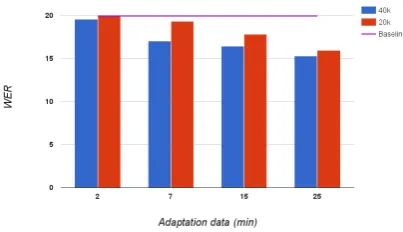
The results in Figure 1 show that the MAP adaptation improves the SI model for ”Speaker1”, even if the model size is also reduced. The blue bars represent WER after the normal MAP adap-tation when the model size remains unchanged. The red bars show WER when the model is com-pressed during the adaptation. The purple hori-zontal line represents the performance of the
Figure 1: WER comparison of the normally MAP adapted (40k) and compressed model (20k) for ”Speaker 1”, where the numbers indicate the num-ber of Gaussian components.
line SI model without any adaptations. The WER for the baseline was 19.93%. Figure 1 shows that
as the adaptation set increases the accuracy im-proves with both methods and the difference in WER between the compressed and the uncom-pressed model reduces. The results were similar with the other speakers as well, as can be seen from the tables 1 and 2.
The improvement of the compressed models could be explained by the MAP estimates converg-ing towards the SD model estimates as the adapta-tion data increases. The WER for ”Speaker1” with the SD model was 10.02%. The results also imply
that all the SI model components are not necessary for all users.
It was also experimented with the ”Speaker1” if similar results could be achieved by using the ML estimates instead of the MAP estimates in com-pression. However, as can be seen from Table 3, the ML estimates do not improve the accuracy of the SI model, which had WER 19.93%, until the
adaptation data has reached 25 minutes.
Table 1:Uncompressed MAP (WER).
Adaption set
SI 2 min 7 min 15 min 25 min Speaker1 19.93 19.58 17.00 16.42 15.28 Speaker2 27.40 23.30 22.80 23.30 22.20 Speaker3 29.7 30.20 28.90 28.00 27.30
Table 2:Compressed MAP (WER).
Adaption set
SI 2 min 7 min 15 min 25 min Speaker1 19.93 19.94 19.30 17.84 15.95 Speaker2 27.40 24.10 21.00 21.00 18.90 Speaker3 29.7 34.70 30.00 27.80 26.30
Table 3:WER for ”Speaker1” after adapting with ML estimates.
Adaption set
SI SD 2 min 7 min 15 min 25 min
WER 19.93 10.02 25.19 21.40 20.55 19.76
4 Discussion
While the initial experiments were repeated for three quite different speakers and texts, trying even more speakers will be the obvious way to verify the conclusions. Non-standard test speakers, such as non-natives, elderly, children and those having speaking disorders will be particularly interesting to observe.
The initial acoustic model was a relatively large and robust SI model. With a smaller SI model, the behavior of the method could be different. Smaller models should compress more moderately than larger models, since the occupancy of the adap-tation set is allocated to fewer model components and relatively more components achieve the mini-mum occupancy value.
The models were compressed by half in the ex-periments after a single iteration. It is however possible to use multiple iterations to reduce the size further. However, compressing the model too much without a sufficient amount of adaptation data could result a loss of important components and the accuracy would decrease. At the moment, the only way to control the amount of compres-sion is to adjust the minimum occupancy threshold for merging. Unfortunately, this approach is lim-ited as after the adaptation many components will have zero occupancy. The next step is to explore the optimal amount of compression and if different merging algorithms could provide better results.
The mean of each Gaussian has so far been the only parameter adapted in the experiments. The WER could be improved more rapidly by updating the other HMM parameters as well (Sharma and Hasegawa-Johnson, 2010).
can be used in combination with other compres-sion and adaptation methods, because it directly modifies the Gaussian parameters. We success-fully adapted a discriminatively trained SI model with our method, as well. The results were simi-lar with the ML SI model we presented in this pa-per. This implies that compressing MAP adapta-tion can be combined with a variety of techniques. The usability of the speech recognition applica-tion depends on the accuracy and latency of the ASR system. Hence, the model size is crucial, since high complexity causes latency to the ASR system. Currently, large SI models dominate in the applications as they suit for many acoustic en-vironments. However, it is easier to accomplish higher accuracy with an ASR system trained for a limited acoustic environment. With small personal devices there is no need for a large SI model, as they typically have a single user. If the models are small enough, it is possible to run the ASR system and store the model locally in the device. Utilizing the memory of the device would reduce the mem-ory demand on the server. One possible applica-tion for our method would be to adapt and com-press the SI model during the use and to move the models completely into the user’s device, when the models are small enough.
5 Conclusions
The MAP adaptation was expanded with split and merge operations which are used in ML training. The initial results indicate that the method can compresses the SI model by a half while still im-proving the performance with the speaker adapta-tion. While the results are promising, more ex-periments are required to confirm that our method is suitable for the personalization of the acoustic model.
Acknowledgments
This work was supported by Academy of Finland with the grant 251170, Nokia Inc. and the Founda-tion for Aalto University Science and Technology with the post-graduate grant, and Aalto Science-IT project by providing the computational resources.
References
Enrico Bocchieri and Brian Kan-Wing Mak. 2001. Subspace Distribution Clustering Hidden Markov Model. Speech and Audio Processing, IEEE Trans-actions on, 9(3):264–275.
David F. Crouse, Peter Willett, Krishna Pattipati, and Lennart Svensson. 2011. A look at Gaussian mix-ture reduction algorithms. In Information Fusion (FUSION), 2011 Proceedings of the 14th Interna-tional Conference.
Jean-Luc Gauvain and Chin-Hui Lee. 1994. Max-imum a posteriori estimation for multivariate Gaussian mixture observations of Markov chains.
Speech and audio processing, ieee transactions on, 2(2):291–298.
Geoffrey Hinton, Li Deng, Dong Yu, George E Dahl, Abdel-rahman Mohamed, Navdeep Jaitly, Andrew Senior, Vincent Vanhoucke, Patrick Nguyen, Tara N Sainath, et al. 2012. Deep Neural Networks for acoustic modeling in speech recognition: The shared views of four research groups. Signal Processing Magazine, IEEE, 29(6):82–97.
Teemu Hirsimaki, Janne Pylkkonen, and Mikko Ku-rimo. 2009. Importance of high-order n-gram models in morph-based speech recognition. Audio, Speech, and Language Processing, IEEE Transac-tions on, 17(4):724–732.
Xuedong Huang and Kai-Fu Lee. 1993. On independent, dependent, and speaker-adaptive speech recognition. IEEE Transactions on Speech and Audio processing, 1(2):150–157. Xuedong Huang, Alex Acero, Hsiao-Wuen Hon, and
Raj Foreword By-Reddy. 2001. Spoken language processing: A guide to theory, algorithm, and system development. Prentice Hall PTR.
Mei-Yuh Hwang and Xuedong Huang. 1993. Shared-distribution Hidden Markov Models for speech recognition. Speech and Audio Processing, IEEE Transactions on, 1(4):414–420.
Dorota J Iskra, Beate Grosskopf, Krzysztof Marasek, Henk van den Heuvel, Frank Diehl, and Andreas Kiessling. 2002. SPEECON-Speech databases for consumer devices: Database specification and vali-dation. InLREC.
Christopher J Leggetter and Philip C Woodland. 1995. Maximum Likelihood Linear Regression for speaker adaptation of continuous density Hidden Markov Models. Computer Speech & Language, 9(2):171– 185.
Harsh Vardhan Sharma and Mark Hasegawa-Johnson. 2010. State-transition interpolation and MAP adap-tation for HMM-based dysarthric speech recogni-tion. InProceedings of the NAACL HLT 2010 Work-shop on Speech and Language Processing for As-sistive Technologies, pages 72–79. Association for Computational Linguistics.
Steve Young, Gunnar Evermann, Mark Gales, Thomas Hain, Dan Kershaw, Xunying Liu, Gareth Moore, Julian Odell, Dave Ollason, Dan Povey, et al. 1997.