Supertagging with LSTMs
Ashish Vaswani1, Yonatan Bisk1, Kenji Sagae2, and Ryan Musa3 1University of Southern California,2Kitt.ai
3University of Illinois at Urbana-Champaign
[email protected], [email protected] [email protected], [email protected]
Abstract
In this paper we present new state-of-the-art performance on CCG supertagging and pars-ing. Our model outperforms existing ap-proaches by an absolute gain of 1.5%. We an-alyze the performance of several neural mod-els and demonstrate that while feed-forward architectures can compete with bidirectional LSTMs on POS tagging, models that encode the complete sentence are necessary for the long range syntactic information encoded in supertags.
1 Introduction
Morphosyntactic labels for words are commonly used in a variety of NLP applications. For this rea-son, part-of-speech (POS) tagging and supertagging have drawn significant attention from the commu-nity. Combinatory Categorial Grammar is a lexical-ized grammar formalism that is widely used for syn-tactic and semantic parsing. Supertagging (Clark, 2002; Bangalore and Joshi, 2010) assigns complex syntactic labels to words to enable fast and accurate parsing. The disambiguation of correctly labeling a word with one of over 1,200 CCG labels is dif-ficult compared to choosing on of the 45 POS la-bels in the Penn Treebank (Marcus et al., 1993). In addition to the large label space of CCG supertags, labeling a word correctly depends on knowledge of syntactic phenomena arbitrarily far in the sentence (Hockenmaier and Steedman, 2007). This is be-cause supertags encode highly specific syntactic in-formation (e.g. types and locations of arguments) about a word’s usage in a sentence.
In this paper, we show that Bidirectional Long Short-Term Memory recurrent neural networks (bi– LSTMs) (Graves, 2013; Zaremba et al., 2014), which can use information from the entire sentence,
are a natural and powerful architecture for CCG su-pertagging. In addition to the bi–LSTM, we create a simple yet novel model that outperforms the pre-vious state-of-the-art RNN model that uses hand-crafted features (Xu et al., 2015) by 1.5%. Con-current to this work (Lewis et al., 2016) introduced a different training methodology for bi-LSTM for supertagging. We provide a detailed analysis of the quality of various LSTM architectures, forward, backward, and bi-directional, shedding light over the ability of the bi–LSTM to exploit rich sentential con-text necessary for performing supertagging. We also show that a baseline feed-forward neural network (NN) architecture significantly outperforms previ-ous feed-forward NN baselines, with slightly fewer features, achieving better accuracy than the RNN model from (Xu et al., 2015).
Recently, bi–LSTMs have achieved high accu-racies in a simpler sequence labeling task: part-of-speech tagging (Wang et al., 2015; Ling et al., 2015) on the Penn treebank, with small improve-ments over local models. However, we achieve strong accuracies compared to (Wang et al., 2015) using feed-forward neural network model trained on local context, showing that this task does not require bi–LSTMs. Our strong feed-forward NN baselines show the power of feed-forward NNs for some tasks.
Our main contributions are the introduction of a new bi–LSTM model for CCG supertagging that achieves state-of-the-art, on both CCG supertagging and parsing, and a detailed analysis of our results, including a comparison of bi–LSTMs and simpler feed forward NN models for supertagging and POS tagging, which suggests that the added complexity of bi–LSTMs may not be necessary for POS tagging, where local contexts suffice to a much greater extent than in supertagging.
2 Models And Training
We use feed-forward neural network models and bidirectional LSTM (bi–LSTM) based models in this work.
2.1 Feed-Forward
For both POS tagging and our baseline supertagging model, we use feed-forward neural networks with two hidden layers of rectified linear units (Nair and Hinton, 2010). For supertagging, we use a slightly smaller set than Lewis and Steedman (2014a), us-ing a left and right 3-word window with suffix and capitalization features for the center word. However, unlike them, we train on the full set of supertag cat-egories observed during training.
In POS tagging, when tagging wordwi, we
con-sider only features from a window of five words, with wi at the center. For each wj with i−2 ≤
j ≤ i+ 2, we add wj lowercased and a string that
encodes the basic “word shape” ofwj. This is
com-puted by replacing all sequences of uppercase letters withA, all sequences of lowercase letters witha, all sequences of digits with9, and all sequences of other characters with∗. Finally, we add two and three let-ter suffixes and two letlet-ter prefix forwionly.
2.2 LSTM models
We experiment with two kinds of bi–LSTM models. We train a basic bi–LSTM where the forward and backward LSTMs take input wordswi and produce
hidden state−→hi and←−hi. For each position, we
pro-duce˜hi, where ˜
hi=σ(W←−h←−hiT +W−→h−→hTi ), (1)
where σ(x) = max(0, x) is a rectifier nonlinear-ity, and where W←−h and W−→h are parameters to be learned. The unnormalized likelihood of an output supertag is computed using supertag embeddings
Dti and biasesbti asp(ti |h˜i) =Dti˜hTi +bti. The final softmax layer computes normalized supertag probabilities.
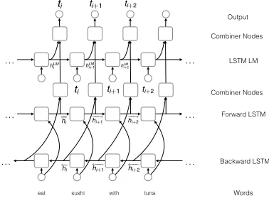
Although bidirectional LSTMs can capture long distance interactions between words, each output la-bel is predicted independently. To explicitly model supertag interactions, our next model combines two models, the bi–LSTM and a LSTM language model (LM) over the supertags (Figure 1). At position
… …
… …
…
Backward LSTM Forward LSTM Combiner Nodes
LSTM LM Combiner Nodes
Output
Words hLM
i hLMi+1 hLM i
+2
←−hi ←−−h i+1 ←−−hi+2
−−→
hi+2
−−→ hi+1 − →h i
ti ti+1 ti+2
ti ti+1 ti+2
…
[image:2.612.329.518.66.209.2]eat sushi with tuna
Figure 1:We add a language model between supertags.
i, the LM accepts an input supertag ti−1 produc-ing hidden statehLM
i , and a second combiner layer,
parametrized by matricesWLM andW˜h transforms
˜
hi and hLMi to hi similar to the combiner for ˜hi
(Equation 1). Output supertag probabilities are com-puted just as before, replacing replacing˜hi withhi.
We refer to this model as bi–LSTM–LM. For all our LSTM models, we only use words as input features.
2.3 Training
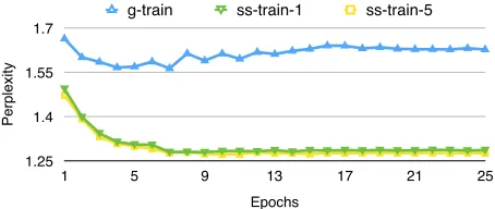
We train our models to maximize the log-likelihood of the data with minibatch gradient ascent. Gradi-ents of the models are computed with backpropa-gation (Chauvin and Rumelhart, 1995). Since gold supertags are available during training time and not while decoding, a bi–LSTM–LM trained on gold su-pertags might not recover from errors caused by us-ing incorrectly predicted supertags. This results in the bi–LSTM–LM slightly underperforming the bi– LSTM (we refer to training with gold supertags as g–train in Table 1). To bridge this gap between train-ing and testtrain-ing we also experiment with a sampltrain-ing training regime in addition to training.
Epoch g-train SS-train-1b SS-train-kb 11.663079261779785 1.493532538414001 1.471613883972168 2 1.59983241558075 1.397878646850586 1.391600012779236 31.584500551223755 1.343078851699829 1.331377267837524 41.565570712089539 1.313792586326599 1.307917714118958
51.568343997001648 1.305177807807922 1.298569440841675 61.585107803344727 1.30352258682251 1.290364503860474 71.562329530715942 1.279528975486755 1.276203751564026 81.612882614135742 1.2797691822052 1.279410839080811 91.588557481765747 1.278935551643372 1.273308753967285 101.612249255180359 1.28274667263031 1.272010803222656
111.594677925109863 1.282948136329651 1.272024273872375 121.617396116256714 1.281896352767944 1.278515696525574 131.610980749130249 1.285645723342896 1.274761080741882 141.621490359306335 1.28062105178833 1.275495886802673 151.628495216369629 1.285783290863037 1.272665500640869
161.639569163322449 1.284226417541504 1.276064276695251 171.638893842697144 1.286049485206604 1.275808334350586 181.630186915397644 1.284650564193726 1.275925874710083 191.633984208106995 1.286053538322449 1.276958823204041 201.628738522529602 1.284542202949524 1.27592945098877 211.627252221107483 1.284929633140564 1.276000380516052
221.627161264419556 1.28664767742157 1.276474475860596 231.626600503921509 1.2862898111343381.275714635848999 241.630642294883728 1.284499049186707 1.275835752487183 251.626240372657776 1.285952687263489 1.275785207748413
Pe
rp
le
xi
ty
1.25 1.4 1.55 1.7
Epochs
1 5 9 13 17 21 25
g-train ss-train-1 ss-train-5
[image:3.612.72.299.60.156.2]1
Figure 2: Scheduled sampling improves the perplexity of the gold sequence under predicted tags. We see that the perplexity of the gold supertag sequence when using predicted tags for the LM is lower for ss–train–1 and ss–train–5 than with g–train.
use their probabilities (re-normalized over the5-best tags) and scale the input supertag embeddings with their re-normalized probability during look-up. We refer to this setting as ss–train–5. In this work, we use an inverse sigmoid schedule to computep,
p= k
k+esk,
where s is the epoch number and k is a hyperpa-rameter that is tuned.1 In Figure 2, we see that for
the development set training with scheduled sam-pling improves the perplexity of the gold supertag sequence when using predicted supertags, indicat-ing better recovery from conditionindicat-ing on erroneous supertags. For both ss-train and g-train, we use gold supertags for the output layer and train the model to maximize the log-likelihood of the data.2
2.4 Architectures
Our feed-forward models use2048rectifier units in the first hidden layer,50and128rectifier units in the second hidden layer for POS tagging and Supertag-ging respectively, and 64 dim. input embeddings.
Our LSTM based models use 512hidden states. We pre-train our word embeddings with a 7 -gram feed-forward neural language model using the NPLM toolkit3on a concatenation of the BLLIP
cor-pus (Charniak et al., 2000) and WSJ sections 02–21 of the Penn Treebank.
1The reader should refer to (Bengio et al., 2015) for details. 2We use dropout for all our feed-forward (Srivastava, 2013)
and bi-LSTM based models (Zaremba et al., 2014). We carry out a grid search over dropout probabilities and sampling sched-ules. We train the LSTMs for25epochs and the feed-forward models for30epochs, tuning on the development data.
3http://nlg.isi.edu/software/nplm/
Supertag Accuracy
Model All Seen Novel % P
Lewis et al. (2014) 91.30
Wenduan et al. (2015) 93.07
Feed Forward + g–train 93.29 93.77 91.53 70.3
Forward LSTM + g–train 83.70 85.76 46.22 20.7
Backward LSTM + g–train 88.82 90.06 66.22 40.6
bi–LSTM 94.08 95.03 76.36 81.1
bi–LSTM–LM + g–train 93.89 94.93 76.83 96.5
[image:3.612.314.542.64.209.2]bi–LSTM–LM + ss–train–1 94.24 95.22 76.70 87.8 bi–LSTM–LM + ss–train–5 94.23 95.20 76.62 94.5
Table 1:Accuracies on the development section. The language model provides a boost in performance, and large gains on the parseability of the sequence (%P). The numbers for bi–LSTM– LM + ss–train–1 and + g–train are with beam decoding. All others use greedy decoding. Interestingly, greedy decoding with ss–train–5 works as well as beam decoding with ss–train–1.
2.5 Decoding
We perform greedy decoding. For each positioni, we select the most probable supertag from the output distribution. For the bi–LSTM–LM models trained with g–train and ss–train–1, we feed the most likely supertag from the output distribution as LM input in the next position. We decode with beam search (size 12) for bi–LSTM–LMs trained with g–train and ss–train–1. For the bi–LSTM–LMs trained with ss–train–5, we perform greedy decoding similar to training, feeding thek-best supertags from the out-put supertag distribution in positioni−1 as input to the LM in position i, along with the renormal-ized probabilities. We don’t perform beam decoding for ss–train–5, as the previousk-best inputs already capture different paths through the network.4
3 Data
For supertagging, experiments were run with the standard splits of CCGbank. Unlike previous work no features were extracted for the LSTM models and rare categories were not thresholded. Words were lowercased and digits replaced with @.
CCGbank’s training section contains 1,284 lexi-cal categories (394 in Dev). The distribution of gories has a long tail, with only a third of those
cate-4Code and supertags for our models can be downloaded
LSTM
Supertag F-For Forward Backward bi–LSTM +LM(g–train) ss–train–1 ss–train–5
(NP\NP)/NP 90.00 88.89 81.91 92.09 92.18 91.72 92.31
((S\NP)\(S\NP))/NP 75.75 69.53 61.60 80.38 78.21 79.91 78.77
S[dcl]\NP 77.29 61.14 58.52 84.28 83.41 82.97 80.35
(S[dcl]\NP)/NP 91.39 56.58 69.86 92.34 92.46 92.46 92.82
((S[dcl]\NP)/PP)/NP 42.30 30.77 42.31 56.41 64.10 62.82 60.26
(S[dcl]\NP)/(S[adj]\NP) 86.80 22.84 83.25 87.31 88.83 87.82 86.80
((S[dcl]\NP)/(S[to]\NP))/NP 86.49 56.76 75.68 94.59 91.89 91.89 91.89
Table 2:Prediction accuracy for our models on several common and difficult supertags.
Architecture Test Acc Ling et al. (2015) Bi-LSTM 97.36 Wang et al. (2015) Bi-LSTM 97.78
Søgaard (2011) SCNN 97.50
This work Feed-Forward 97.40
Table 3: Our new POS tagging results show a strong Feed-Forward baseline can perform as well as or better than more sophisticated models (e.g. Bi-LSTMs).
gories having a frequency count≥10(the threshold used by existing literature). Following (Lewis and Steedman, 2014b), we allow the model to predict all categories for a word, not just those with which the word was observed to co-occur in the training data. Accuracies on these unseen (word, cat) pairs are pre-sented in the third column of Table 1.
4 Results
Table 3 presents our Feed-Forward POS tagging re-sults. We achieve 97.28% on the development set and 97.4% on test. Although slightly below state-of-the-art, we approach existing work with bi–LSTMs, and our models are much simpler and faster to train.5
Table 1 shows a steady increase in performance as the model is provided additional context. The for-ward and backfor-ward models are presented with infor-mation that may be arbitrarily far away in the sen-tence, but only in a specific direction. This yields weaker results than the Feed Forward model which can see in both directions within a small window. The real gains are achieved by the Bidirectional LSTM which incorporates knowledge from the en-tire sentence. Our addition of a language model and changes to training, further improve the
perfor-5We use train, dev, and test splits of WSJ sections 00–18,
19–21, and 22–24, for POS tagging.
Dev F1 Test F1 Wenduan et al. (2015) 86.25 87.04 + new POS Tags & C&C 86.99 87.50 bi–LSTM–LM +ss–train–1 87.75 88.32
Table 4:Parsing at 100% coverage with our new Feed-Forward POS tagger and the Java implementation of C&C. We show both the published and improved results for Wenduan et al.
mance. Our final model (bi–LSTM–LM+ss–train–1 model with beam decoding) has a test accuracy of 94.5%, 1.5% above state-of-the-art.
4.1 Parsing
Our primary goal in this paper was to demonstrate how a bi–LSTM captures new and different in-formation from uni-directional or feed-forward ap-proaches. This advantage also translates to gains in parsing. Table 4 presents new state-of-the-art parsing results for both (Xu et al., 2015) and our bi–LSTM–LM +ss–train–1. These results were at-tained using our part-of-speech tags (Table 3) and the Java implementation (Clark et al., 2015) of the C&C parser (Clark and Curran, 2007)6.
4.2 Error Analysis
Our analysis indicates that the information follow-ing a word is more informative than what preceded it. Table 2 compares how well our models recover common and syntactically interesting supertags. In particular, the Forward and Backward models, moti-vate the need for a Bi-directional approach.
6Results are presented on the standard development and test
splits (Section 00 and 23), and with a beam threshold of10−6.
(S[dcl]\NP)/(S[adj]\NP)
Forward Backward Bidirectional
((S[dcl]\NP)/PP)/(S[adj]\NP) ((S[dcl]\NP)/PP)/(S[adj]\NP) (S[dcl]\NP)/(S[pss]\NP)
((S[dcl]\NP)/(S[to]\NP))/(S[adj]\NP) ((S[b]\NP)\NP)/(S[adj]\NP) (S[dcl]\NP)/PP)/(S[adj]\NP)
((S[dcl]\NP)/PP)/PP (S[dcl]\S[qem])/(S[adj]\NP) (S[b]\NP)\NP)/(S[adj]\NP)
(S[dcl]\NP)/S ((S[dcl]\NP)/(S[to]\NP))/(S[adj]\NP) (S[dcl]\NP)/(S[to]\NP))/(S[adj]\NP)
(S[dcl]\NP)/(S[pss]\NP) ((S[dcl]\NP)/(S[adj]\NP))/(S[adj]\NP) (S[dcl]\NP)/(S[adj]\NP))/(S[adj]\NP)
Table 5:“Neighbor” categories as determined by embedding-based vector similarity for each class of model. As expected for this category, the Backward model captures the argument preference while the Forward model correctly predicts the result.
The first two rows show prepositional phrase at-tachment decisions (noun and verb attaching cate-gories are in rows one and two, respectively). Here the forward model outperforms the backward model, presumably because knowing the word to be modi-fied and the preposition, is more important than ob-serving the object of the prepositional phrase (the information available to the backward model).
Conversely, the backward model outperforms the forward model in most of the remaining categories. (Di-)transitive verbs (lines 4 & 5) require knowledge of future arguments in the sentence (e.g. separated by a relative clause). Because English has strict SVO word-order, the presence of a subject is more pre-dictable than the presence of an (in-)direct object. It is therefore not surprising that the backward model is often comparable to the Feed Forward model.
If the information missing from either the forward or backward models were local, the bidirectional model should perform the same as the Feed-Forward model, instead it surpasses it, often by a large mar-gin. This implies there is long range information necessary for choosing a supertag.
Embeddings In addition, we can visualize the in-formation captured by our models by investigating a category’s nearest neighbors based on the learned embeddings. Table 5 shows nearest neighbor cate-gories for(S[dcl]\NP)/(S[adj]\NP)under the For-ward, BackFor-ward, and Bidirectional models.
We see see that the forward model learns inter-nal structure with the query category, but the list of arguments is nearly random. In contrast, the back-ward model clusters categories primarily based on the final argument, perhaps sharing similarities in the subject argument only because of the predictable SVO nature of English text. However, due to its lack of forward context the model incorrectly
asso-ciates categories with less-common first arguments (e.g.S[qem]). Finally, the bidirectional embeddings appear to cleanly capture the strengths of both the forward and backward models.
Consistency and Internal Structure Because su-pertags are highly structured their co-occurence in a sentence must be permitted by the combinators of CCG. Without encoding this explicitly, the lan-guage model dramatically increases the percent of predicted sequences that result in a valid parse by up to 15% (last column of Table 2).
Sparsity One consideration of our approach is that we do not threshold rare categories or use any tag dictionaries; our models are presented with the full space of CCG categories, despite the long tail. This did not did not hurt performance and the models learned to successfully use several categories which were outside the set of traditionally-thresholded fre-quent categories. Additionally, the total number of categories used correctly at least once by the bi-directional models was substantially higher than the other models (∼270 vs. ∼220 of 394), though the large number of unused categories (≥120) indicates that there is still substantial room for improvement.
5 Conclusions and Future Work
Because bi–LSTMs with a language model encode an entire sentence at decision time, we demonstrated large gains in supertagging and parsing. Future work will investigate improving performance on rare cat-egories.
Acknowledgements
References
Srinivas Bangalore and Aravind K. Joshi. 2010. Su-pertagging: Using Complex Lexical Descriptions in Natural Language Processing. The MIT Press. Samy Bengio, Oriol Vinyals, Navdeep Jaitly, and Noam
Shazeer. 2015. Scheduled sampling for sequence pre-diction with recurrent neural networks. InAdvances in Neural Information Processing Systems, pages 1171– 1179.
Eugene Charniak, Don Blaheta, Niyu Ge, Keith Hall, John Hale, and Mark Johnson. 2000. Bllip 1987-89 wsj corpus release 1. Linguistic Data Consortium, Philadelphia, 36.
Yves Chauvin and David E Rumelhart. 1995. Backprop-agation: theory, architectures, and applications. Psy-chology Press.
Stephen Clark and James Curran. 2007. Wide-Coverage Efficient Statistical Parsing with CCG and Log-Linear Models.Computational Linguistics, 33(4):493–552. Stephen Clark, Darren Foong, Luana Bulat, and Wenduan
Xu. 2015. The Java Version of the C&C Parser: Ver-sion 0.95. Technical report, University of Cambridge Computer Laboratory, August.
Stephen Clark. 2002. Supertagging for combinatory cat-egorial grammar. InProceedings of the 6th Interna-tional Workshop on Tree Adjoining Grammars and Re-lated Formalisms (TAG+6), pages 19–24.
A. Graves. 2013. Generating sequences with recurrent neural networks. arXiv preprint arXiv:1308.0850. Julia Hockenmaier and Mark Steedman. 2007.
CCG-bank: A Corpus of CCG Derivations and Dependency Structures Extracted from the Penn Treebank. Com-putational Linguistics, 33:355–396, September. Mike Lewis and Mark Steedman. 2014a. A* ccg
pars-ing with a supertag-factored model. InProceedings of the Conference on Empirical Methods in Natural Lan-guage Processing (EMNLP-2014).
Mike Lewis and Mark Steedman. 2014b. Improved ccg parsing with semi-supervised supertagging. Transac-tions of the Association for Computational Linguistics, 2:327–338.
Mike Lewis, Kenton Lee, and Luke Zettlemoyer. 2016. LSTM CCG Parsing. InProceedings of the 15th An-nual Conference of the North American Chapter of the Association for Computational Linguistics.
Wang Ling, Tiago Luís, Luís Marujo, Ramón Fernan-dez Astudillo, Silvio Amir, Chris Dyer, Alan W Black, and Isabel Trancoso. 2015. Finding func-tion in form: Composifunc-tional character models for open vocabulary word representation. arXiv preprint arXiv:1508.02096.
Mitchell P Marcus, Beatrice Santorini, and Mary Ann Marcinkiewicz. 1993. Building a Large Annotated
Corpus of English: The Penn Treebank. Computa-tional Linguistics, 19:313–330, June.
Vinod Nair and Geoffrey E. Hinton. 2010. Rectified lin-ear units improve restricted Boltzmann machines. In Proceedings of ICML, pages 807–814.
Marc’Aurelio Ranzato, Sumit Chopra, Michael Auli, and Wojciech Zaremba. 2015. Sequence Level Train-ing with Recurrent Neural Networks. arXiv preprint arXiv:1511.06732.
Anders Søgaard. 2011. Semisupervised condensed near-est neighbor for part-of-speech tagging. In Proceed-ings of the 49th Annual Meeting of the Association for Computational Linguistics: Human Language Tech-nologies: short papers-Volume 2, pages 48–52. Asso-ciation for Computational Linguistics.
Nitish Srivastava. 2013.Improving neural networks with dropout. Ph.D. thesis, University of Toronto.
Peilu Wang, Yao Qian, Frank K Soong, Lei He, and Hai Zhao. 2015. Part-of-speech tagging with bidirec-tional long short-term memory recurrent neural net-work. arXiv preprint arXiv:1510.06168.
Wenduan Xu, Michael Auli, and Stephen Clark. 2015. Ccg supertagging with a recurrent neural network. Volume 2: Short Papers, page 250.