Count-Invariance Including Exponentials
Stepan Kuznetsov
Steklov Mathematical Institute (Moscow), RAS
Glyn Morrill
Universitat Polit`ecnica de Catalunya [email protected]
Oriol Valent´ın
Universitat Polit`ecnica de Catalunya [email protected]
Abstract
We define infinitary count-invariance for categorial logic, extending
count-invariance for multiplicatives (van
Benthem,1991) and additives and bracket modalities (Valent´ın et al., 2013) to include exponentials. This provides an effective tool for pruning proof search in
categorial parsing/theorem-proving.
1 Introduction
In logical grammar, which dates back to (
Aj-dukiewicz,1935), grammar isreducedto logic: an expression is grammatical if and only if an associ-ated logical statement is a theorem of a calculus.
1.1 Sharing
In standard logic information does not have mul-tiplicity. Thus where + is the notion of addition
of information and≤is the notion of inclusion we
have x+x ≤ xandx ≤ x+x; both these two
prop-erties together amount to idempotency: x+x = x.
These properties are expressed by the rules of in-ference of Contraction and Expansion:
(1) a. ∆(A,A)⇒BContraction
∆(A)⇒B
b. ∆(A)⇒B Expansion
∆(A,A)⇒B
Linguistic resources do not freely have these prop-erties: grammaticality is not generally preserved under addition or removal of copies of words or expressions. However, there are some construc-tions manifesting something similiar. Parasitic gaps involve a kind of Contraction. Parasitic gaps cannot occur anywhere, thus:
(2) *the slave thatiJohn soldei toei
Rather, we assume here that as the term ‘parasitic’ suggests, a parasitic gap must fall within an is-land. Extraction from weak islands can become fully acceptable when accompanied by a cobound non-island extraction:
(3) a. man thati[the friends ofei] admireei
b. paper thatiJohn filedei[without
readingei]
c. paper thati[the editor ofei] filedei
[without readingei]
And iterated coordination allows a kind of Expan-sion:
(4) John likes, Mary dislikes and Bill loves Lon-don.
That is, in logical grammar a controlled use of
idempotency, or sharing, is motivated. Girard
(1987) introduced exponentials for such control. Versions of the exponentials have been used to treat (parasitic) gaps and iterated coordination and iterated “respectively” in categorial gram-mar (Morrill,2017), (Morrill and Valent´ın,2015a,
2016b).
1.2 Count-Invariance
Count-invariance for multiplicatives in (sub)linear logic is introduced invan Benthem(1991). This involves simply checking the number of positive and negative occurrences of each atom in a se-quent. Thus where #(Σ) is a count of the sequent
Σwe have:
(5) `Σ =⇒#(Σ)=0
I.e. the numbers of positive and negative occur-rences of each atom must exactly balance for the sequent to be a theorem. This provides a neces-sary, but of course not sufficient, criterion for
the-oremhood, and can be checked rapidly. It can be
used as a filter in proof search: if backward chain-ing proof search generates a goal which does not satisfy the count-invariant, the goal can be dis-carded. This notion of count for multiplicatives
was included in the categorial parser/
theorem-prover CatLog (Morrill,2012).
InValent´ın et al.(2013) the idea is extended to additives (and bracket modalities). Instead of a single count for each atom of a sequentΣwe have
a minimum count #min(Σ) and a maximum count
#max(Σ) and for a sequent to be a theorem it must
satisfy two inequations:
(6) `Σ =⇒#min(Σ)≤0≤#max(Σ)
I.e. the count functions #min and #max define an interval which must include the point of balance
0; for the multiplicatives, #min = #max = # and
(6) reduces to the special case (5). This gener-alised notion of count is included in the categorial parser/theorem-prover CatLog2.
The structure of the continuation of the paper is as follows. In Section2 we present the infini-tary count algebra which we employ, we define the fragment of categorial logic for which we il-lustrate count invariance, and we define the (in-finitary) count functions for this fragment. In Sec-tion3we state and prove our count-invariance the-orem. In Section4we evaluate the introduction of exponential count invariance experimentally in re-lation to CatLog parsing/theorem-proving.
2 Infinitary Count Algebra
We consider terms built over constants 0, 1,
⊥(−∞: minus infinity), and>(+∞: plus infinity)
by binary operations of plus (+), minus (−),
minimum (min) and maximum (max), and the infinitary step functionsXandY as follows where iand jare integers (* indicates undefined):
+ j ⊥ >
i i+j ⊥ > ⊥ ⊥ ⊥ ∗ > > ∗ >
− j ⊥ >
i i−j > ⊥
⊥ ⊥ ∗ ⊥
> > > ∗
min j ⊥ >
i |i+j|−|2i−j| ⊥ i
⊥ ⊥ ⊥ ⊥
> j ⊥ >
max j ⊥ >
i |i+j|+|i−j|
2 i >
⊥ j ⊥ >
> > > >
X(i)=
(
> ifi>0
i ifi≤0
Y(i)=
(
i ifi≥0
⊥ ifi<0
(7) Proposition. 0. ⊥ < i< >; 1. fora,b < >, a+b< >; 2. fora,b> ⊥,a+b >⊥; 3. for a>⊥&b<>,b−a<>; 4. forb>⊥&a<
>,b−a>⊥; 5. fora,b>⊥, min(a,b)>⊥& max(a,b)>⊥; 6. fora,b<>, min(a,b)<> & max(a,b)<>; 7. fora>⊥,X(a) >⊥; 8. fora<>,Y(a)<>.
2.1 The count functions
The count function, or count functions, are func-tions from types and sequents into values in the count algebra such that if sequents are provable their images under the count functions fall within a certain range. It follows that if their images do notfall within the required range then the sequents arenotprovable; we give examples after defining the count functions, in the next subsection. This provides an efficient filter on parsing/
theorem-proving, as we show in the last section.
Let us assume primitive types P. For Q ∈
P∪{[]}, m ∈ {min,max} and min = max and
max=min we define
#m,Q(Γ⇒A)=#◦m,Q(A)−#•m,Q(Γ)
where #◦ and #• are as below. We define the
en-richment LAb!b? of the Lambek calculus (
Lam-bek,1958) with typesTpas follows:
Tp ::= P |
Tp\Tp|Tp/Tp|Tp•Tp|
Tp&Tp|Tp⊕Tp|
[ ]−1Tp| hiTp| !Tp|?Tp
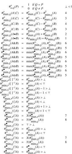
define the count functions:
#mp,Q(P) = 1 ifQ=P
0 ifQ,P
#mp,Q(A\C) = #mp,Q(C)−#mp,Q(A)
#mp,Q(C/B) = #mp,Q(C)−#mp,Q(B)
#mp,Q(A•B) = #mp,Q(A)+#mp,Q(B)
#◦m,Q(A&B) = m(#◦m,Q(A),#◦m,Q(B)) #•m,Q(A&B) = m(#m•,Q(A),#•m,Q(B))
#◦m,Q(A⊕B) = m(#◦m,Q(A),#◦m,Q(B))
#•m,Q(A⊕B) = m(#•m,Q(A),#•m,Q(B))
#mp,P([ ]−1A) = #p m,P(A)
#mp,[]([ ]−1A) = #p
m,[](A)−1 #mp,P(hiA) = #mp,P(A)
#mp,[](hiA) = #mp,[](A)+1
#◦m,Q(!A) = #◦m,Q(A)
#•min
,Q(!A) = Y(#•min,Q(A))
#•max,P(!A) = X(#•max,P(A))
#•max,[](!A) = >
#◦min
,Q(?A) = Y(#◦min,Q(A))
#◦max,Q(?A) = X(#◦max,Q(A))
#•m,Q(?A) = #•m,Q(A)
(8) Lemma. #pm(A) is defined and ⊥ <
#max(A) & #min(A)<>.
Proof. By induction as in Figure1; justifications
refer to the Proposition (7).
To present sequents we define configurations
Configandtree termsTreeTermin terms of types
Tpas follows, whereΛis the empty string:
Config ::= Λ|TreeTerm,Config
TreeTerm ::= Tp|[Config]
The rules forLAb!b? are shown in Figure2. Note
that !Cis of a generalised form necessary to prove Cut-elimination in the presence of !R. Note also that ?Lis an infinitary rule; it is not used in linguis-tic applications. We include it here for the sake of showing technical completeness of the count in-variance. For tree terms and configurations, counts are:
#•m,Q(Γ,∆) = #•m,Q(Γ)+#•m,Q(∆)
#•m,P([Γ]) = #•m,P(Γ)
#•m,[]([Γ]) = #•m,[](Γ)+1
#•m,Q(Λ) = 0
Lemma8extends to configurations.
2.2 Examples
Relativisation including medial and parasitic ex-traction is obtained by assigning a relative
pro-noun a type (CN\CN)/(!N\S) whereby the body
of a relative clause is analysed as !N\S. By
way of example of count-invariance, we show how it discardsN,N\S ⇒!N\S corresponding to the ungrammaticality of a relative clause
with-out a gap: *paper that John walks. We have
the max N-count: #max,N(N,N\S ⇒!N\S) =
#◦max,N(!N\S)−#•min
,N(N,N\S) = #◦max.N(S)−
#•min
,N(!N) − #•min,N(N) − #•min,N(N\S) = 0 −
Y(#•min
,N(N)) − 1 − #•min,N(S) + #◦min,N(N) = −Y(1)−1−0+1= −1−1+1 =−1 6≥ 0 which
means that the count-invariance is not satisfied.
Iterated sentential coordination is
ob-tained by assigning a coordinator the type
(?S\S)/S. By way of a second
exam-ple we show how count-invariance discards
N,N,N\S ⇒?S corresponding to the
un-grammaticality of unequilibrated coordination:
*John Mary walks and Suzy talks. Max N-count
is: #max,N(N,N,N\S ⇒?S) = #◦max,N(?S) −
#•min,N(N,N,N\S) = X(#◦max,N(S)) −
#•min,N(N) − #•min,N(N) − #•min,N(N\S) =
X(0) − 1 − 1 − #•min
,N(S) + #•max,N(N) =
0− 2− 0+ 1 = −1 6≥ 0 which means that the
count-invariance is not satisfied.
3 Theorem and Proof Our main theorem is:
(9) Theorem.
`Γ⇒A=⇒ ∀Q∈ P ∪ {[]},
#min,Q(Γ⇒A)≤0≤#max,Q(Γ⇒A)
where as we have said,
#m,Q(Γ⇒A)=#◦m,Q(A)−#•m,Q(Γ).
Proof. The proof is by induction on the length
of derivations. For the base caseP⇒Pwe have
#m,Q(P⇒P)=#◦m,Q(P)−#•m,Q(P)=0. The
induc-tive cases are as follows, where we use:
• a+b=b+a
• a+(b+c)=(a+b)+c
• a−(b+c)=(a−b)−c(including the undefined
case)
#mp,Q(P) = 1 ifQ=P
0 ifQ,P ⊥<0,1<>
#maxp ,Q(A\C) = #pmax,Q(C)−#minp
,Q(A) 4
#minp
,Q(A\C) = # p
min,Q(C)−# p
max,Q(A) 3
#maxp ,Q(C/B) = #pmax,Q(C)−#minp
,Q(B) 4
#pmin
,Q(C/B) = #
p
min,Q(C)−# p
max,Q(B) 3
#maxp ,Q(A•B) = #maxp ,Q(A)+#pmax,Q(B) 2
#minp
,Q(A•B) = #pmin,Q(A)+#pmin,Q(B) 1
#◦min
,Q(A&B) = max(#◦min,Q(A),#◦min,Q(B)) 6
#◦max,Q(A&B) = min(#◦max,Q(A),#◦max,Q(B)) 5
#•min
,Q(A&B) = min(#•min,Q(A),#•min,Q(B)) 6
#•max,Q(A&B) = max(#max• ,Q(A),#•max,Q(B)) 5
#◦min
,Q(A⊕B) = min(#◦min,Q(A),#◦min,Q(B)) 6
#◦max,Q(A⊕B) = max(#◦max,Q(A),#◦max,Q(B)) 5
#•min
,Q(A⊕B) = max(#•min,Q(A),#•min,Q(B)) 6
#•max,Q(A⊕B) = min(#max• ,Q(A),#•max,Q(B)) 5 #maxp ,P([ ]−1A) = #p
max,P(A)>⊥
#minp ,P([ ]−
1A) = #p
min,P(A)<>
#maxp ,[]([ ]−1A) = #p
max,[](A)−1>⊥ #minp ,[]([ ]−1A) = #p
min,[](A)−1<> #maxp ,P(hiA) = #pmax,P(A)>⊥
#minp
,P(hiA) = # p
min,P(A)<⊥
#maxp ,[](hiA) = #pmax,[](A)+1>⊥ #minp ,[](hiA) = #pmin
,[](A)+1<>
#•max,P(!A) = X(#•max,P(A)) 7
#•min
,Q(!A) = Y(#•min,Q(A)) 8
#•max,[](!A) = >>⊥
#◦max,Q(!A) = #◦max,Q(A)>⊥ #◦min
,Q(!A) = #◦min,Q(A)<>
#◦max,Q(?A) = X(#◦max,Q(A)) 7
#◦min
,Q(?A) = Y(#◦min,Q(A)) 8
#•min
,Q(?A) = #•min,Q(A)<>
[image:4.595.158.408.128.661.2]#•max,Q(?A) = #•max,Q(A)>⊥
id,P∈ P
P⇒P
Γ⇒A ∆(C)⇒D
\L
∆(Γ,A\C)⇒D
Γ⇒B ∆(C)⇒D
\L
∆(C/B,Γ)⇒D
A,Γ⇒C
\R
Γ⇒A\C
Γ,B⇒C
/R
Γ⇒C/B
∆(A,B)⇒C
•L
∆(A•B)⇒C
Γ1⇒A Γ2⇒B
•R
Γ1,Γ2⇒A•B
∆(A)⇒D
&L1
∆(A&B)⇒D
∆(B)⇒D
&L2
∆(A&B)⇒D
Γ⇒A Γ⇒B
&R
Γ⇒A&B
Γ⇒A
⊕R1
Γ⇒A⊕B
Γ⇒B
⊕R2
Γ⇒A⊕B
∆(A)⇒D ∆(B)⇒D
⊕L
∆(A⊕B)⇒D
Γ(A)⇒B
[ ]−1L
Γ([[ ]−1A])⇒B
[Γ]⇒A
[ ]−1R
Γ⇒[ ]−1A
Γ([A])⇒B
hiL
Γ(hiA)⇒B
Γ⇒A
hiR [Γ]⇒ hiA
∆(A)⇒D
!L
∆(!A)⇒D
!A1, . . . ,!An⇒A
!R !A1, . . . ,!An⇒!A
∆(Γ,!A)⇒D
!P1
∆(!A,Γ)⇒D
∆(!A,Γ)⇒D
!P2
∆(Γ,!A)⇒D
∆(!A0, . . . ,!An,[!A0, . . . ,!An,Γ])⇒D
!C
∆(!A0, . . . ,!An,Γ)⇒D
∆(A)⇒D ∆(A,A)⇒D . . . ?L
∆(?A)⇒D
Γ⇒A
?R
Γ⇒?A
Γ1⇒C Γ2⇒?C
?M
[image:5.595.122.483.160.639.2]Γ1,Γ2⇒?C
• a−(b−c)=(a−b)+c
(Where we write #(∆) with∆a context we should
more precisely understand that∆is a configuration
with a hole where the count of a hole is always zero.)
Multiplicatives
• Γ⇒A ∆(C)⇒D\L
∆(Γ,A\C)⇒D
For every atom or bracket,
#m(∆(Γ,A\C)⇒D)=
#◦m(D)−#•m(∆)−#•m(Γ)−#•m(A\C)=
#◦m(D)−#•m(∆)−#m•(Γ)−#•m(C)+#◦m(A)=
#◦m(A)−#•m(Γ)+#m◦(D)−#•m(∆)−#•m(C)=
#m(Γ⇒A)+#m(∆(C)⇒D)
The induction hypothesis (i.h.) tells us that
#min(Γ⇒A)≤ 0 and #min(∆(C)⇒D)≤ 0.
Thus #min(∆(Γ,A\C)⇒D) = #min(Γ⇒A) +
#min(∆(C)⇒D)≤ 0. Similarly,
0≤ #max(∆(Γ,A\C)⇒D) = #max(Γ⇒A) +
#max(∆(C)⇒D) byi.h.Therefore we have:
#min(∆(Γ,A\C)⇒D)≤0≤ #max(∆(Γ,A\C)⇒D)
• Γ⇒B ∆(C)⇒D\L
∆(C/B,Γ)⇒D
Like\L.
• A,Γ⇒C \R
Γ⇒A\C
For every atom or bracket,
#m(Γ⇒A\C)=
#◦m(A\C)−#•m(Γ)=
#◦m(C)−#•m(A)−#•m(Γ)=
#m(A,Γ⇒C)
Therefore byi.h.,
#min(Γ⇒A\C)≤0≤#max(Γ⇒A\C)
• Γ,B⇒C/R
Γ⇒C/B
Like\R.
• ∆(A,B)⇒C •L
∆(A•B)⇒C
For every atom or bracket,
#m(∆(A•B)⇒C)=
#◦m(C)−#•m(∆)−#•m(A•B)=
#◦m(C)−#•m(∆)−#•m(A)−#•m(B)=
#m(∆(A,B)⇒C)
Therefore byi.h.,
#min(∆(A•B)⇒C)≤0≤
#max(∆(A•B)⇒C)
• Γ1⇒A Γ2⇒B•R
Γ1,Γ2⇒A•B
For every atom or bracket,
#m(Γ1,Γ2⇒A•B)= #◦m(A•B)−#m•(Γ1,Γ2)=
#◦m(A)−#•m(Γ1)+#◦m(B)−#•m(Γ2)=
#m(Γ1⇒A)+#m(Γ2⇒B) Therefore byi.h.,
#min(Γ1,Γ2⇒A•B)≤0≤ #max(Γ1,Γ2⇒A•B)
Additives
• ∆(A)⇒D &L1
∆(A&B)⇒D
For every atom or bracket,
#min(∆(A&B)⇒D)=
#◦min(D)−#•max(∆)−#•max(A&B)=
#◦min(D)−#•max(∆)−
max(#•max(A),#•max(B))≤
#◦min(D)−#•max(∆)−#•max(A)=
#max(∆(A&B)⇒D)=
#◦max(D)−#•min(∆)−#•min(A&B)=
#◦max(D)−#•min(∆)−
min(#•min(A),#•min(B))≥
#◦max(D)−#•min(∆)−#•min(A)=
#max(∆(A)⇒D)≥0i.h.
Therefore:
#min(∆(A&B)⇒D)≤0≤
#max(∆(A&B)⇒D)
• ∆(B)⇒D &L2
∆(A&B)⇒D
Like &L1.
• Γ⇒A Γ⇒B&R
Γ⇒A&B
#min(Γ⇒A&B)=
#◦min(A&B)−#•max(Γ)=
max(#◦min(A),#◦min(B))−#•max(Γ)=
max(#◦min(A)−#•max(Γ),
#◦min(B)−#•max(Γ))=
max(#min(Γ⇒A)
| {z }
≤0i.h.
,#min(Γ⇒B) | {z }
≤0i.h. )
| {z }
≤0 And
#max(Γ⇒A&B)=
#◦max(A&B)−#•min(Γ)=
min(#◦max(A),#◦max(B))−#•min(Γ)=
min(#◦max(A)−#•min(Γ), #◦max(B)−#•min(Γ))=
min(#max(Γ⇒A)
| {z }
0≤ i.h.
,#max(Γ⇒B)
| {z }
0≤ i.h. )
| {z }
0≤ Therefore:
#min(Γ⇒A&B)≤0≤ #max(Γ⇒A&B).
• Γ⇒A ⊕R1
Γ⇒A⊕B
#min(Γ⇒A⊕B)=
#◦min(A⊕B)−#•max(Γ)=
min(#◦min(A),#•min(B))−#•max(Γ)≤
#◦min(A)−#•max(Γ)=
#min(Γ⇒A)≤0i.h.
And
#max(Γ⇒A⊕B)=
#◦max(A⊕B)−#•min(Γ)=
max(#•max(A),#•max(B))−#•min(Γ)≥
#•max(A)−#•min(Γ)=
#max(Γ⇒A)≥0i.h.
• Γ⇒B ⊕R2
Γ⇒A⊕B
Like⊕R1.
• ∆(A)⇒D ∆(B)⇒D⊕L
∆(A⊕B)⇒D
For every atom or bracket,
#min(∆(A⊕B)⇒D)=
#◦min(D)−#•max(∆)−#•max(A⊕B)=
#◦min(D)−#•max(∆)−
min(#•max(A),#•max(B))=
max(#◦min(D)−#•max(∆)−#•max(A),
#◦min(D)−#•max(∆)−#•max(B))=
max(#min(∆(A)⇒D)
| {z }
≤0i.h.
,#min(∆(B)⇒D) | {z }
≤0i.h. )
| {z }
≤0
0≤#max(∆(A⊕B)⇒D) similarly
Bracket modalities
• Γ(A)⇒B [ ]−1L
Γ([[ ]−1A])⇒B
For atoms:
#m,P(Γ([[ ]−1A])⇒B)=
#◦m,P(B)−#m•,P(Γ([[ ]−1A]))=
#◦m,P(B)−#•m,P(Γ)−#•m,P([[ ]−1A]))=
#◦m,P(B)−#•m,P(Γ)−#•m,P([ ]−1A))=
#◦m,P(B)−#•m,P(Γ)−#•m,P(A))=
#◦m,P(B)−#•m,P(Γ(A))=
#m,P(Γ(A)⇒B)
I.e. the property for the conclusion follows from the induccion hypothesis for the premise since brackets and bracket modalities are transparent to atom count.
#m,[](Γ([[ ]−1A])⇒B)= #◦m,[](B)−#•m,[](Γ([[ ]−1A]))=
#◦m,[](B)−#•m,[](Γ)−#•m,[]([[ ]−1A]))=
#◦m,[](B)−#•m,[](Γ)−#•m,[]([ ]−1A)−1=
#◦m,[](B)−#•m,[](Γ)−#•m,[](A)+1−1=
#◦m,[](B)−#•m,[](Γ)−#•m,[](A))=
#◦m,[](B)−#•m,[](Γ(A))=
#m,[](Γ(A)⇒B)= Therefore byi.h.,
#min(Γ([[ ]−1A])⇒B)≤0≤
#max(Γ([[ ]−1A])⇒B)
• [Γ]⇒A [ ]−1R
Γ⇒[ ]−1A
For atoms:
#m,P(Γ⇒[ ]−1A)=
#m,P(Γ⇒A)=
#m,P([Γ]⇒A)
Since brackets and bracket modalities are transparant to atom count.
For brackets:
#m,[](Γ⇒[ ]−1A)=
#◦m,[]([ ]−1A)−#•
m,[](Γ)= #◦m,[](A)−1−#•m,[](Γ)=
#◦m,[](A)−(#•m,[](Γ)+1)=
#◦m,[](A)−#•m,[]([Γ])=
#m,[]([Γ]⇒A)
Therefore byi.h.
#min(Γ⇒[ ]−1A)≤0≤#max(Γ⇒[ ]−1A)
• Γ([A])⇒BhiL
Γ(hiA)⇒B
For atoms,
#m,P(Γ(hiA)⇒B)=#m,P(Γ([A])⇒B)
since brackets and bracket modalities are trans-parent to atom count.
For brackets,
#m,[](Γ(hiA)⇒B)=
#◦m,[](B)−#•m,[](Γ)−#•m,[](hiA)=
#◦m,[](B)−#•m,[](Γ)−(#•m,[](A)+1)=
#◦m,[](B)−#•m,[](Γ)−#•m,[]([A])=
#m,[](Γ([A])⇒B) Therefore byi.h.
#min(Γ(hiA)⇒B)≤0≤#max(Γ(hiA)⇒B)
• Γ⇒A hiR [Γ]⇒ hiA
For atoms,
#m,P([Γ]⇒ hiA)=#m,P(Γ⇒A)
since brackets and bracket modalities are trans-parent to atom count.
For brackets,
#m,[]([Γ]⇒ hiA)= #◦m,[](hiA)−#•m,[]([Γ])=
#◦m,[](A)+1−#•m,[](Γ)−1=
#◦m,[](A)−#•m,[](Γ)=
#m,[](Γ⇒A)
Therefore byi.h.:
#min([Γ]⇒ hiA)≤0≤#max([Γ]⇒ hiA)
3.1 Exponentials
• ∆(A)⇒D !L
∆(!A)⇒D
For atoms,
#min,P(∆(!A)⇒D)=
#◦min
,P(D)−#•max,P(∆)−#•max,P(!A)=
#◦min
,P(D)−#•max,P(∆)−X(#•max,P(A))≤
#◦min,P(D)−#•max,P(∆)−#•max,P(A)=
#min,P(∆(A)⇒D)≤0i.h.
#min,[](∆(!A)⇒D)=
#◦min,[](D)−#•max,[](∆)−#•max,[](!A)=
#◦min,[](D)−#•max,[](∆)− > ≤
#◦min,[](D)−#•max,[](∆)−#•max,[](A)=
#min,[](∆(A)⇒D)≤0i.h. For atoms and brackets,
#max,Q(∆(!A)⇒D)=
#◦max,Q(D)−#•min
,Q(∆)−#•min,Q(!A)=
#◦max,Q(D)−#•min
,Q(∆)−Y(#•min,Q(A))≥
#◦max,Q(D)−#•min
,Q(∆)−#•min,Q(A)=
#max,Q(∆(A)⇒D)≥0i.h.
• !A1, . . . ,!An⇒A !R !A1, . . . ,!An⇒!A
For atoms,
#m,P(!A1, . . . ,!An⇒!A)=
#◦m,P(!A)−#m•,P(!A1, . . . ,!An)=
#◦m,P(A)−#m•,P(!A1, . . . ,!An)=
#m,P(!A1, . . . ,!An⇒A)
For brackets,
#m,[](!A1, . . . ,!An⇒!A)=
#◦m,[](!A)−#m•,[](!A1, . . . ,!An)=
#◦m,[](A)−#m•,[](!A1, . . . ,!An)=
#◦m,[](A)−#m•,[](!A1, . . . ,!An)=
#m,[](!A1, . . . ,!An⇒A)≥0i.h.
• ∆(!A0, . . . ,!An,[!A0, . . . ,!An,Γ])⇒D!C
∆(!A0, . . . ,!An,Γ)⇒D
For atoms,
#min(∆(!A0, . . . ,!An,Γ)⇒D)=
#◦min(D)−#•max(∆,Γ)
−#•max(!A0)− · · · −#•max(!An)=
#◦min(D)−#•max(∆,Γ)
−X(#•max(A0))− · · · −X(#•max(An))≤
#◦min(D)−#•max(∆,[Γ])−
X(#•max(A0))− · · · −X(#•max(An))−
X(#•max(A0))− · · · −X(#•max(An))=
#min(∆(!A0, . . . ,!An,|
[!A0, . . . ,!An,Γ])⇒D)≤0
For brackets,
#min(∆(!A0, . . . ,!An,Γ)⇒D)=
#◦min(D)−#•max(∆,Γ)
−#•max(!A0)− · · · −#•max(!An)=
#◦min(D)−#•max(∆,Γ)− > − · · · − > ≤
#◦min(D)−#•max(∆,[Γ])− > − · · · − >− > − · · · − >=
#min(∆(!A0, . . . ,!An,
[!A0, . . . ,!An,Γ])⇒D)≤0
And for atoms and brackets,
#max(∆(!A0, . . . ,!An,Γ)⇒D)=
#◦max(D)−#•min(∆,Γ)
−#•min(!A0)− · · · −#•min(!An)=
#◦max(D)−#•min(∆,Γ)
−Y(#•min(A0))− · · · −Y(#•min(An))≥
#◦max(D)−#•min(∆,[Γ])−
Y(#•min(A0))− · · · −Y(#•min(An))−
Y(#•min(A0))− · · · −Y(#•min(An))=
#max(∆(!A0, . . . ,!An,
[!A0, . . . ,!An,Γ])⇒D)≥0
• ∆(A)⇒D ∆(A,A)⇒D. . .?L
∆(?A)⇒D
For atoms and brackets,
#min(∆(?A)⇒D)=
#◦min(D)−#•max(∆)−#•max(?A)=
#◦min(D)−#•max(∆)−X(#•max(A))≤
#◦min(D)−#•max(∆)−#•max(A)=
#min(∆(A)⇒D)≤0i.h. And
#max(∆(?A)⇒D)=
#◦max(D)−#•min(∆)−#•min(?A)=
#◦max(D)−#•min(∆)−Y(#•min(A))≥
#◦max(D)−#•min(∆)−#•min(A)=
#max(∆(A)⇒D)≥0i.h.
• Γ⇒A ?R
Γ⇒?A
For atoms and brackets,
#min(Γ⇒?A)=
#◦min(?A)−#•max(Γ)=
Y(#◦min(A))−#•max(Γ)≤
#◦min(A)−#•max(Γ)=
And,
#max(Γ⇒?A)=
#◦max(?A)−#•min(Γ)=
X(#◦max(A))−#•min(Γ)≥
#◦max(A)−#•min(Γ)=
#◦max(Γ⇒A)
• Γ⇒A ∆⇒?A?M
Γ,∆⇒?A
For atoms and brackets,
#min(Γ,∆⇒?A)=
#◦min(?A)−#•max(Γ)−#•max(∆)=
Y(#◦min(A))−#•max(Γ)−#•max(∆)≤
Y(#◦min(A))+#◦min(A)−#•max(Γ)−#•max(∆)=
#◦min(A)−#•max(Γ) | {z }
≤0i.h.
+#◦min(?A)−#•max(∆) | {z }
≤0i.h.
| {z }
≤0 And,
#max(Γ,∆⇒?A)=
#◦max(?A)−#•min(Γ)−#•min(∆n)=
X(#◦max(A))−#•min(Γ)−#•min(∆)≥
X(#◦max(A))+#◦max(A))−#•min(Γ)−#•min(∆)=
#◦max(A)−#•min(Γ) | {z }
≥0i.h.
+#◦max(?A)−#•min(∆) | {z }
≥0i.h.
| {z }
≥0
4 Evaluation
By way of evaluation of the exponential count in-variance we compared the performance of Cat-Log2 (version f8.1) which uses only multiplicative and additive count invariance with CatLog version j2 which uses in addition the exponential
invari-ance,1both running under XGP Prolog on a
Mac-Book Air. The lexicon was the same in both cases. We timed individually the exhaustive parsing of the expressions in Figure3. Thus, for the sentence a:
(10) [john]+likes+the+man:S f there is the result of lexical lookup:
(11) [Nt(s(m)) :j],
((hi∃gNt(s(g))\S f)/∃aNa) :
ˆλAλB(Pres((ˇlike A)B)),
1The engines are otherwise the same.
∀n(Nt(n)/CNn) :ι,
CNs(m) :man ⇒ S f
Note that these types include, in addition to the Lambek connectives, normal modalities for
intensionality — for rigid designators and
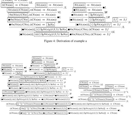
for semantically active intensionality— and first-order quantifiers for features; these connectives are transparent to count-invariance. There is the derivation given in Figure4, which delivers logi-cal form:
(12) (Pres((ˇlike(ιˇman))j))
CatLog proceeds by focalised proof search (
Mor-rill and Valent´ın,2015b). The focusing discipline considerably reduces redundancy in the sequent proof search space. The focusing discipline com-prises alternating phases of invertible rule appli-cation and focalised non-invertible rule
applica-tion. The boxes in the derivations mark the
fo-cusedtypes in focused rule application, i.e. the
ac-tive types decomposed by non-invertible rule ap-plications. The focusing constrains proof search but in displaying proofs the boxes are limited to this decorative role.
For the sentence d:
(13) man+[[that+[john]+likes]] :CNs(m)
there is the lexical lookup:
(14) CNs(m) :man,
[[∀n([]−1[]−1(CNn\CNn)/((hiNt(n)u
!Nt(n))\S f)) :λAλBλC[(B C)∧(A C)],
[Nt(s(m)) :j],
((hi∃gNt(s(g))\S f)/∃aNa) :
ˆλDλE(Pres((ˇlike D)E))]] ⇒ CNs(m)
Note that these types include also an additive and an exponential which are subject to the count-invariance presented in this paper. There is the derivation given in Figure5. This uses stoups for the sequent derivation with exponentials (Girard,
2011), (Morrill,2017). It delivers the logical form:
(15) λC[(ˇman C)∧(Pres((ˇlike C)j))]
a. John likes the man.
b. Mary thinks that John likes the man.
c. Suzy believes that Mary thinks that John likes the man. d. man that John likes
e. man that Mary thinks that John likes
f. man that Suzy believes that Mary thinks that John likes
g. Mary talks and Bill sings.
h. John walks Mary talks and Bill sings.
i. Suzy laughs John walks Mary talks and Bill sings.
j. Bill walks Suzy laughs John walks Mary talks and Bill sings.
k. Suzy talks Bill walks Suzy laughs John walks Mary talks and Bill sings.
[image:11.595.77.528.322.449.2]l. John sings Suzy talks Bill walks Suzy laughs John walks Mary talks and Bill sings.
Figure 3: Example sentences
CNs(m) ⇒ CNs(m)
L
CNs(m) ⇒ CNs(m) Nt(s(m)) ⇒ Nt(s(m)) /L Nt(s(m))/CNs(m),CNs(m) ⇒ Nt(s(m))
∀L ∀n(Nt(n)/CNn),CNs(m) ⇒ Nt(s(m))
L
∀n(Nt(n)/CNn),CNs(m) ⇒ Nt(s(m))
∃R
∀n(Nt(n)/CNn),CNs(m) ⇒ ∃aNa
Nt(s(m)) ⇒ Nt(s(m))
L
Nt(s(m)) ⇒ Nt(s(m))
∃R
Nt(s(m)) ⇒ ∃gNt(s(g))
hiR
[Nt(s(m))] ⇒ hi∃gNt(s(g)) S f ⇒ S f \L
[Nt(s(m))], hi∃gNt(s(g))\S f ⇒ S f
/L [Nt(s(m))], (hi∃gNt(s(g))\S f)/∃aNa,∀n(Nt(n)/CNn),CNs(m) ⇒ S f
L
[image:11.595.71.530.326.725.2][Nt(s(m))], ((hi∃gNt(s(g))\S f)/∃aNa),∀n(Nt(n)/CNn),CNs(m) ⇒ S f
Figure 4: Derivation of example a
Nt(s(m)) ⇒ Nt(s(m)) L
Nt(s(m)) ⇒ Nt(s(m)) ∃R
Nt(s(m))⇒ ∃aNa
Nt(s(m)) ⇒ Nt(s(m)) L
Nt(s(m)) ⇒ Nt(s(m)) ∃R
Nt(s(m)) ⇒ ∃gNt(s(g)) hiR
[Nt(s(m))] ⇒ hi∃gNt(s(g)) S f ⇒ S f
\L
[Nt(s(m))], hi∃gNt(s(g))\S f ⇒ S f
/L
[Nt(s(m))],(hi∃gNt(s(g))\S f)/∃aNa,Nt(s(m))⇒ S f
L
[Nt(s(m))],((hi∃gNt(s(g))\S f)/∃aNa),Nt(s(m)) ⇒ S f
!P
Nt(s(m)) ; [Nt(s(m))],((hi∃gNt(s(g))\S f)/∃aNa)⇒ S f
!L
!Nt(s(m)),[Nt(s(m))],((hi∃gNt(s(g))\S f)/∃aNa) ⇒ S f
uL
hiNt(s(m))u!Nt(s(m)),[Nt(s(m))],((hi∃gNt(s(g))\S f)/∃aNa)⇒ S f
\R
[Nt(s(m))],((hi∃gNt(s(g))\S f)/∃aNa) ⇒ (hiNt(s(m))u!Nt(s(m)))\S f
R
[Nt(s(m))],((hi∃gNt(s(g))\S f)/∃aNa) ⇒((hiNt(s(m))u!Nt(s(m)))\S f)
CNs(m) ⇒CNs(m) L
CNs(m) ⇒ CNs(m) CNs(m) ⇒ CNs(m) \L
CNs(m), CNs(m)\CNs(m) ⇒CNs(m) []−1L CNs(m),[ []−1(CNs(m)\CNs(m)) ] ⇒ CNs(m)
[]−1L CNs(m),[[ []−1[]−1(CNs(m)\CNs(m)) ]]⇒ CNs(m)
/L
CNs(m),[[ []−1[]−1(CNs(m)\CNs(m))/((hiNt(s(m))u!Nt(s(m)))\S f),[Nt(s(m))],((hi∃gNt(s(g))\S f)/∃aNa)]] ⇒ CNs(m) ∀L
CNs(m),[[∀n([]−1[]−1(CNn\CNn)/((hiNt(n)u!Nt(n))\S f)),[Nt(s(m))],((hi∃gNt(s(g))\S f)/∃aNa)]] ⇒ CNs(m) L
CNs(m),[[∀n([]−1[]−1(CNn\CNn)/((hiNt(n)u!Nt(n))\S f)),[Nt(s(m))],((hi∃gNt(s(g))\S f)/∃aNa)]] ⇒ CNs(m)
[image:11.595.73.532.525.724.2](16) f8.1 j2 (no exp. inv) (exp. inv)
a. 1 1
b. 2 2
c. 40 6
d. 2 2
e. 4 4
f. 265 6
g. 1 1
h. 2 1
i. 2 1
j. 2 2
k. 2 3
l. 2 4
We see that for the longer, third, example of a-c there is a speedup. This is mostly in the time taken to discard inappropriate lexical choices (e.g.
thatis lexically ambiguous between a
complemen-tiser and a relative pronoun): to show that there are no further analyses. The examples d-f involve the universal exponential in a relative pronoun roughly of the form (CN\CN)/((hiNu!N)\S); the (semantically inactively) additively conjoined hy-pothetical subtypes are for subject relativisation and object relativisation respectively (Morrill,
2017). Again we see a considerable speedup with
exponential count invariance in the longer third case. The examples g-l involve the existential ex-ponential in a coordinator assignment roughly of the form (?S\[ ]−1[ ]−1S)/S to obtain the iteration. Here there is no gain from the exponential type in-variance; the overhead causes a slowdown.
For the minicorpus examples of the Montague
Test(Morrill and Valent´ın,2016a), and for the full CatLog2 corpus (Montague minicorpus, typical categorial examples, discontinuity examples, rel-ativisation and coordination examples, and some Scripture) the parsing times in seconds were:
(17) f8.1 j2
Montague Test. 37 32
CatLog2 corpus 826 643
We interpret the experiment as showing that the pruning of the search space of count-invariance in-cluding exponentials outweighs the overhead that it engenders: it delivers a speedup of around 20%.
Acknowledgements
SK supported by RFBR. GM supported by an ICREA Academia 2012. GM and OV supported by MINECO TIN2014-57226-P (APCOM).
References
K. Ajdukiewicz. 1935. Die syntaktische Konnexit¨at.
Studia Philosophica 1:1–27. Translated in S. Mc-Call, editor, 1967,Polish Logic: 1920–1939, Oxford University Press, Oxford, 207–231.
J.-Y. Girard. 1987. Linear logic.Theoretical Computer Science50:1–102.
J.-Y. Girard. 2011. The Blind Spot. European Mathe-matical Society, Z¨urich.
J. Lambek. 1958. The mathematics of sentence struc-ture. American Mathematical Monthly65:154–170.
G. Morrill. 2012. CatLog: A Categorial Parser/Theorem-Prover. In LACL 2012 System Demonstrations. Nantes, Logical Aspects of Computational Linguistics 2012, pages 13–16.
G. Morrill. 2017. Grammar logicised: relativisation.
Linguistics and Philosophy40(2):119–163.
G. Morrill and O. Valent´ın. 2015a. Computational Coverage of TLG: Nonlinearity. In M. Kanazawa, L.S. Moss, and V. de Paiva, editors, Proceedings of NLCS’15. Third Workshop on Natural Language and Computer Science. Kyoto, volume 32 ofEPiC, pages 51–63.
G. Morrill and O. Valent´ın. 2015b. Multiplicative-Additive Focusing for Parsing as Deduction. In I. Cervesato and C. Sch¨urmann, editors,First Inter-national Workshop on Focusing, LPAR 2015. Suva, Fiji, number 197 in EPTCS, pages 29–54.
G. Morrill and O. Valent´ın. 2016a. Computational cov-erage of Type Logical Grammar: The Montague Test. In C. Pi˜n´on, editor,Empirical Issues in Syntax and Semantics, Colloque de Syntaxe et S´emantique `a Paris, Paris, volume 11, pages 141–170.
G. Morrill and O. Valent´ın. 2016b. On the Logic of Expansion in Natural Language. In M. Amblard, P. de Groote, S. Pogodalla, and C. Retor´e, editors,
Proceedings of Logical Aspects of Computational Linguistics, LACL’16, Nancy. Springer, Berlin, vol-ume 10054 ofLNCS, FoLLI Publications on Logic, Language and Information, pages 228–246.
O. Valent´ın, D. Serret, and G. Morrill. 2013. A Count Invariant for Lambek Calculus with Additives and Bracket Modalities. In G. Morrill and M.-J. Neder-hof, editors,Proceedings of Formal Grammar 2012 and 2013. Springer, Berlin, volume 8036 ofSpringer LNCS, FoLLI Publications in Logic, Language and Information, pages 263–276.