Learning to Embed Words in Context for Syntactic Tasks
Lifu Tu Kevin Gimpel Karen Livescu
Toyota Technological Institute at Chicago, Chicago, IL, 60637, USA {lifu,kgimpel,klivescu}@ttic.edu
Abstract
We present models for embedding words in the context of surrounding words. Such models, which we refer to astoken em-beddings, represent the characteristics of a word that are specific to a given con-text, such as word sense, syntactic cat-egory, and semantic role. We explore simple, efficient token embedding models based on standard neural network archi-tectures. We learn token embeddings on a large amount of unannotated text and eval-uate them as features for part-of-speech taggers and dependency parsers trained on much smaller amounts of annotated data. We find that predictors endowed with to-ken embeddings consistently outperform baseline predictors across a range of con-text window and training set sizes. 1 Introduction
Word embeddings have enjoyed a surge of popu-larity in natural language processing (NLP) due to the effectiveness of deep learning and the avail-ability of pretrained, downloadable models for embedding words. Many embedding models have been developed (Collobert et al., 2011;Mikolov et al.,2013;Pennington et al.,2014) and have been shown to improve performance on NLP tasks, in-cluding part-of-speech (POS) tagging, named en-tity recognition, semantic role labeling, depen-dency parsing, and machine translation (Turian et al., 2010;Collobert et al., 2011; Bansal et al., 2014;Zou et al.,2013).
The majority of this work has focused on a sin-gle embedding for each word type in a vocab-ulary.1 We will refer to these as type embed-1A word type is an entry in a vocabulary, while a word
token is an instance of a word type in a corpus.
dings. However, the same word type can exhibit a range of linguistic behaviors in different contexts. To address this, some researchers learn multiple
embeddings for certain word types, where each embedding corresponds to a distinct sense of the type (Reisinger and Mooney,2010;Huang et al., 2012;Tian et al.,2014). But token-level linguis-tic phenomena go beyond word sense, and these approaches are only reliable for frequent words.
Several kinds of token-level phenomena relate directly to NLP tasks. Word sense disambigua-tion relies on context to determine which sense is intended. POS tagging, dependency parsing, and semantic role labeling identify syntactic categories and semantic roles for each token. Sentiment anal-ysis and related tasks like opinion mining seek to understand word connotations in context.
In this paper, we develop and evaluate models for embedding word tokens. Our token embed-dings capture linguistic characteristics expressed in the context of a token. Unlike type embeddings, it is infeasible to precompute and store all possi-ble (or even a significant fraction of) token em-beddings. Instead, our token embedding models are parametric, so they can be applied on the fly to embed any word in its context.
We focus on simple and efficient token em-bedding models based on local context and stan-dard neural network architectures. We evaluate our models by using them to provide features for downstream low-resource syntactic tasks: Twitter POS tagging and dependency parsing. We show that token embeddings can improve the perfor-mance of a non-structured POS tagger to match the state of the art Twitter POS tagger ofOwoputi et al. (2013). We add our token embeddings to Tweeboparser (Kong et al., 2014), improving its performance and establishing a new state of the art for Twitter dependency parsing.
2 Related Work
The most common way to obtain context-sensitive embeddings is to learn separate embeddings for distinct senses of each type. Most of these meth-ods cluster tokens into senses and learn vectors for each cluster (Vu and Parker, 2016; Reisinger and Mooney,2010;Huang et al.,2012;Tian et al., 2014;Chen et al.,2014;Pi˜na and Johansson,2015; Wu and Giles, 2015). Some use bilingual infor-mation (Guo et al.,2014; ˇSuster et al.,2016; Go-nen and Goldberg,2016), nonparametric methods to avoid specifying the number of clusters ( Nee-lakantan et al.,2014;Li and Jurafsky,2015), topic models (Liu et al., 2015), grounding to Word-Net (Jauhar et al.,2015), or senses defined as sets of POS tags for each type (Qiu et al.,2014).
These “multi-type” embeddings are restricted to modeling phenomena expressed by a single clus-tering of tokens for each type. In contrast, token embeddings are capable of modeling information that cuts across phenomena categories. Further, as the number of clusters grows, learning multi-type embeddings becomes more difficult due to data fragmentation. Instead, we learnparametric
models that transform a type embedding and those of its context words into a representation for the token. While multi-type embeddings require more data for training, parametric models require less.
There is prior work in developing representa-tions for tokens in the context of unsupervised or supervised training, whether with long short-term memory (LSTM) networks (K˚ageb¨ack et al., 2015;Ling et al.,2015;Choi et al.,2016; Mela-mud et al., 2016), convolutional networks ( Col-lobert et al., 2011), or other architectures. How-ever, learning to represent tokens in supervised training can suffer from limited data. We instead focus on learning token embedding models on un-labeled data, then use them to produce features for downstream tasks. So we focus on efficient archi-tectures and unsupervised learning criteria.
The most closely related work consists of ef-forts to train LSTMs to represent tokens in context using unsupervised training objectives.Kawakami and Dyer(2015) use multilingual data to learn to-ken embeddings that are predictive of their trans-lation targets, while Melamud et al. (2016) and Peters et al. (2017) use unsupervised learning with monolingual sentences. We experiment with LSTM token embedding models as well, though we focus on different tasks: POS tagging and
de-pendency parsing. We generally found that very small contexts worked best for these syntactic tasks, thereby limiting the usefulness of LSTMs as token embedding models.
3 Token Embedding Models
We assume access to pretrained type embeddings. Let W denote a vocabulary of word types. For each word typex∈ W, we denote its type embed-ding byvx ∈Rd.
We define a word sequence x = hx1, x2, ..., x|x|i in which each entry xj is a
word type, i.e.,xj ∈ W. We define a word token
as an element in a word sequence. We consider the class of functionsf that take a word sequence xand indexjof a particular token inxand output a vector of dimensionality d0. We will refer to
choices forf(x, j)asencoders.
3.1 Feedforward Encoders
Our first encoder is a basic feedforward neural network that embeds the sequence of words con-tained in a window of text surrounding word j. We use a fixed-size window containing word j, the w0 words to its left, and the w0 words to its
right. We concatenate the vectors for each word type in this window and apply an affine transfor-mation followed by a nonlinearity:
fFF(x, j) =
gW(D)[vxj−w0;vx(j−w0)+1;...;vxj+w0] +b(D)
where g is an elementwise nonlinear function (e.g.,tanh),W(D)is ad0byd(2w0+1)parameter
matrix, semicolon (;) denotes vertical concatena-tion, andb(D) ∈Rd0
is a bias vector. We assume thatx is padded with start-of-sequence and end-of-sequence symbols as needed. The resultingd0
-dimensional token embedding can be transformed by additional nonlinear layers.
This encoder does not distinguish wordj other than by centering the window at its position. It is left to the training objectives to place empha-sis on wordj as needed (see Section3.3). Vary-ingw0 will influence the phenomena captured by
3.2 Recurrent Neural Network Encoders The above feedforward DNN encoder will be brittle with large window sizes. We therefore also consider encoders based on recurrent neu-ral networks (RNNs). RNNs have recently en-joyed a great deal of interest in the deep learn-ing, speech recognition, and NLP communi-ties (Sundermeyer et al.,2012;Graves et al.,2013; Sutskever et al.,2014), most frequently used with “gated” connections like long short-term mem-ory (LSTM) (Hochreiter and Schmidhuber,1997; Gers et al.,2000).
We use an LSTM to encode the sequence of words containing the token and take the final hid-den vector as thed0-dimensional encoding. While
we can use longer sequences, such as the sentence containing the token (Kawakami and Dyer,2015), we restrict the input sequence to a fixed-size con-text window around wordj, so the input is identi-cal to that of the feedforward encoder above. For the syntactic tasks we consider, we did not find large context windows to be helpful.
3.3 Training
We consider unsupervised ways to train the en-coders described above. Throughout training for both models, the type embeddings are kept fixed. We assume that we are given a corpus X = {x(i)}|X|
i=1of unannotated word sequences. One widely-used family of unsupervised crite-ria is that of reconstruction error and its vacrite-riants. These are used when training autoencoders, which use an encoderf to convert the inputxto a vec-tor followed by a decoder g that attempts to re-construct the input from the vector. The typical loss function is the squared difference between the input and reconstructed input. We use a general-ization that is sensitive to the position of elements. Since our primary interest is in learning useful rep-resentations for a particular token in its context, we use a weighted reconstruction error:
lossWRE(f, g,x, j) = |x|
X
i=1
ωikg(f(x, j))i−vxik22 (1) where g(f(x, j))i is the subvector of g(f(x, j))
corresponding to reconstructingvxi, and whereωi
is the weight for reconstructing theith entry. For our feedforward encoder f, we use anal-ogous fully-connected layers in the decoder g, forming a standard autoencoder architecture. To
train the LSTM encoder, we add an LSTM de-coder to form a sequence-to-sequence (“seq2seq”) autoencoder (Sutskever et al.,2014;Li et al.,2015; Dai and Le,2015). That is, we use one LSTM as the encoderf and another LSTM for the decoder g, initializingg’s hidden state to the output off. Since we use the same weighted reconstruction er-ror described above, the decoder must output a sin-gle vector at each step rather than a distribution over word types. So we use an affine transforma-tion on the LSTM decoder hidden vector at each step in order to generate the output vector for each step. Reconstruction error has efficiency advan-tages over log loss here in that it avoids the costly summation over the vocabulary.
4 Qualitative Analysis
Before discussing downstream tasks, we perform a qualitative analysis to show what our token em-bedding models learn.
4.1 Experimental Setup
We train a feedforward DNN token embedding model on a corpus of 300,000 unlabeled English tweets. We use a window size w0 = 3 for the
qualitative results reported here; for downstream tasks below, we will varyw0. For training, we use
our weighted reconstruction error (Eq.1). The en-coder uses one hidden layer of size 512 followed by the token embedding layer of size d0 = 256.
The decoder also uses a single hidden layer of size 512. We use ReLU activations except the final en-coder/decoder layers which use linear activations. In preliminary experiments we compared 3 weighting schemes forωin the objective: for to-ken indexj, “uniform” weighting setsωi = 1for
alli; “focused” setsωj = 2andωi= 1fori6=j;
and “tapered” setsωj = 4,ωj±1 = 3,ωj±2 = 2, and 1 otherwise. The non-uniform schemes place more emphasis on reconstructing the target token, and we found them to slightly outperform uniform weighting. Unless reported otherwise, we use fo-cused weighting for all experiments below.
We train using stochastic gradient descent with momentum for 1 epoch, saving the model that reaches the best objective value on a held-out val-idation set of 3,000 unlabeled tweets. For the type embeddings used as input to our token embedding model, we train 100-dimensional skip-gram em-beddings on 56 million English tweets using the
Q my firstone was like 2 minutes long andhas Q jus listenin 2 mr hudson anddrake crazyness 1 my favplace- was there 2 years ago andam 1 @mentiondeaddddd u go 2 mlk high upn 2 thought itwas more like 2 ... either way, i 2 only acups tho tryin 2 feed the wholefamily 3 tobackup everything from 2 years before i 3 bored on marsi kum down 2 earth ... yupp!! 4 islept for like 2 sec lol .freakin chessy 4 i missyou i trying 2 looking oud mymind girl Q the lines: i am so thrilled about this. may Q fightingoff a headache so i can workon my 1 and work. i am so glad you asked. let 1 imon my phone so i cant seewho @mention 2 i was so excited to sleepin tomorrow 2 did somethings that hurt so i guess iwas doing 3 @mention that is so funny ! iknow which 3 myphone keeps beeping so i know ralphmust 4 little girl! i was so touched when shecalled 4 randomly obsessedwith this song so i bought it
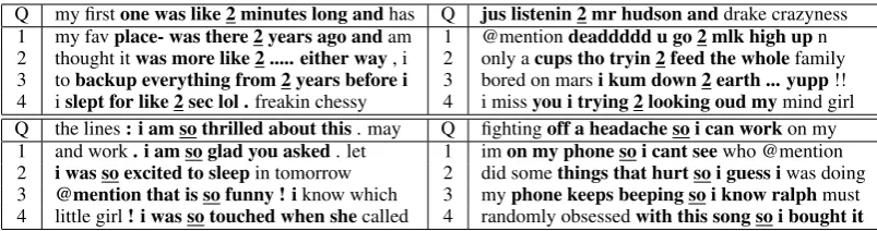
Table 1: Query tokens of two polysemous words and their four nearest neighboring tokens. The target token is underlined and the encoder context (3 words to either side) is shown in bold. See text for details.
4.2 Nearest Neighbor Analysis
We inspect the ability of the encoder to distin-guish different senses of ambiguous types. Table1 shows query tokens (Q) followed by their four nearest neighbor tokens (with the same type), all from our held-out set of 3,000 tweets. We choose two polysemous words that are common in tweets: “2” and “so”. As queries, we select tokens that ex-press different senses. The word “2” can be both a number (left) and a synonym of “to” (right). The word “so” is both an intensifier (left) and a con-nective (right). We find that the nearest neighbors, though generally differing in context words, have the same sense and same POS tag.
In Table 2 we consider nearest neighbors that may have different word types from the query type. For each query word, we permit the near-est neighbor search to consider tokens from the following set: {“4”, “for”, “2”, “to”, “too”, “1”, “one”}. In the first two queries, we find that tokens of “4” have nearest neighbors with different word types but the same syntactic category. That is, to-kens of different word types are more similar to the query than tokens of thesametype. We see this again with neighbors of “2” used as a synonym for “to”. The encoder appears to be doing a kind of canonicalization of nonstandard word uses, which suggests applications for token embeddings in nor-malization of social media text (Clark and Araki, 2011). See neighbor 8, in which “too” is under-stood as having the intended meaning despite its misleading surface form.
4.3 Visualization
In order to gain a better qualitative understand-ing of the token embeddunderstand-ings, we visualize the learned token embeddings using t-SNE (Maaten and Hinton, 2008). We learn token embeddings as above except with w0 = 1. Figure 1 shows
a two-dimensional visualization of token
embed-Q mastersswimmers annual swim 4 your heart !
1 somany miles loking for her and handing
2 off tothe rehearsal space for a weekend long
3 on the inauguration for your enjoyment
Q #canucksnow have a 4 point lead onthe 1 way lol. it’s the 1 mile trail andthen you 2 my firstone was like 2 minutes long and
3 my favplace- was there 2 years ago and
Q jus listenin 2 mr hudson anddrake crazyness 1 @mentiondeaddddd u go 2 mlk high upn bk 2 only acups tho tryin 2 feed the wholefamily 3 are ya’ll listening to the annointed one? he’s on 4 @mention wellcould u come to mrs wilsons for
5 i’m bored on marsi kum down 2 earth ... yupp!! 6 i am listening to amar prtihibi -black
7 aboutneopets and listening to yelle ( URL
8 high riteenow - - bout too troop to thecrib Table 2: Nearest neighbors for token embeddings, where we consider neighbors that may have differ-ent word types from that in the query token. See text for details.
dings for the word type “4”. For this visualiza-tion, we embed tokens in the POS-annotated tweet datasets from Gimpel et al. (2011) and Owoputi et al.(2013), so we have their gold standard POS tags. We show the left and right context words (usingw0 = 1) along with the token and its gold
standard POS tag. We find that tokens of “4” with the same gold POS tag are close in the embed-ded space, with prepositions appearing in the up-per part of the plot and numbers appearing in the lower part.
5 Downstream Tasks
We evaluate our token embedding models on two downstream tasks: POS tagging and depen-dency parsing. Given an input sequence x = hx1, x2, ..., xni, we want to predict its tag
[image:4.595.310.524.211.385.2]1.64
1.66
1.68
1.70
1.72
1.74
4.55
4.60
4.65
4.70
4.75
4.80
wearin 4_P the god 4_P deliverance
effect 4_P <@MENTION>
november 4_$ ??!!
, 4_$ of looking 4_P a
lookn 4_P it
up 4_P no officer 4_P #1
with 4_$ swangas
down 4_P halloween like 4_$ flats
, 4_$ ,
[image:5.595.98.484.98.386.2]<@MENTION> 4_$ pages
Figure 1: t-SNE visualization of token embeddings for word type “4”. Each point shows the left and right context words (w0 = 1) for the token along with the gold standard POS tag following an underscore (“ ”).
The tag “P” is preposition and “$” is number. Following the t-SNE projection, points were subsampled for this visualization for clarity.
5.1 Part-of-Speech Tagging
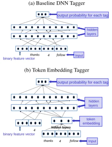
Baseline We use a simple feedforward DNN as our baseline tagger. It is a local classifier that pre-dicts the tag for a token independently of all other predictions for the tweet. That is, it does not use structured prediction. The input to the network is the type embedding of the word to be tagged con-catenated with the type embeddings ofwwords on either side. The DNN contains two hidden layers followed by one softmax layer. Figure2(a) shows this architecture forw= 1when predicting the tag of4in the tweetthanks 4 follow. We concatenate a 10-dimensional binary feature vector computed for the word being tagged (Table3).2
We train the tagger by minimizing the log loss (cross entropy) on the training set, performing early stopping on the validation set, and reporting accuracy on the test set. We consider both learn-ing the type embeddlearn-ings (“updatlearn-ing”) and keeplearn-ing
2The definition of punctuation is taken from Python’s
string.punctuation.
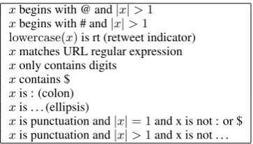
xbegins with @ and|x|>1
xbegins with # and|x|>1
lowercase(x)is rt (retweet indicator) xmatches URL regular expression xonly contains digits
xcontains $ xis : (colon) xis . . . (ellipsis)
xis punctuation and|x|= 1and x is not : or $ xis punctuation and|x|>1and x is not . . .
Table 3: Rules for binary feature vector for word x. If multiple rules apply, the first has priority. The tagger uses this feature vector only for the word to be tagged; the parser uses one for the child and another for the parent in the dependency arc under consideration.
them fixed. When we update the embeddings we include an`2regularization term penalizing the di-vergence from the initial type embeddings.
Token Embedding Tagger When using token embeddings, we concatenate the d0-dimensional
[image:5.595.326.508.466.569.2](a) Baseline DNN Tagger Baseline Tagger
Input hidden layers
output probability for each tag
thanks 4 follow
… …
binary feature vector
(b) Token Embedding Tagger Token Embedding Tagger
Input hidden layers
output probability for each tag
4
… … …
binary feature vector
token embedding
thanks 4 follow
hidden layers
Figure 2: (a) Baseline DNN tagger, (b) tagger aug-mented with token embeddings.
the architecture is the same as the baseline tagger. Figure2(b) shows the model when using type em-bedding window sizew= 0and token embedding window sizew0 = 1.
While training the DNN tagger with the token embeddings, we do not fine-tune the token embed-ding encoder parameters, leaving them fixed.
5.2 Dependency Parser
Baseline As our baseline, we use a simple DNN to do parent prediction independently for each word. That is, we use a local classifier that scores parents for a word. To infer a parse at test time, we independently choose the highest-scoring parent for each word. We also use our classifier’s scores as additional features in Twee-boParser (Kong et al.,2014).
Our parent prediction DNN has two hidden lay-ers and an output layer with 1 unit. This unit corre-sponds to a valueS(xi, xj)that serves as the score
for a dependency arc with child wordxiand parent
wordxj. The input to the DNN is the
concatena-tion of the type embeddings forxiandxj, the type
embeddings of w words on either side of xi and
xj, the features for xi andxj from Table3, and
features for the pair, including relative positions, direction, and distance (shown in Table4).3
3When considering the root attachment (i.e.,x
jis the wall
symbol $), the type embeddings forxjand its neighbors are
all zeroes, the feature vector forxjis all zeroes, and the
de-pendency pair features are all zeroes except the first and last.
For a sentence of lengthn, the loss function we use for a single arc(xi, xj)follows:
lossarc(xi, xj) =
−S(xi, xj) + log
Xn
k=0,k6=i
exp{S(xi, xk)}
(2)
wherek= 0indicates the root attachment forxi.
We sum over all possible parents even though the model only computes a score for a binary deci-sion.4 Wherehead(xi)returns the annotated
par-ent forxi, the loss for a sequencexis: n
X
i=1
lossarc(xi,head(xi)) (3)
After training, we predict the parent for a wordxi
as follows:
head(xi) = argmax
k6=i S(xi, xk) (4)
Token Embedding Parser For the token em-bedding parser, we use the d0-dimensional token
embeddings for xi and xj. We simply
concate-nate the two token embeddings to the input of the DNN parser. Whenxj = $, the token embedding
for xj is all zeroes. The other parts of the input
are the same as the baseline parser. While training this parser, we do not optimize the token embed-ding encoder parameters. As with the tagger, we tune over the decision to keep type embeddings fixed or update them during learning, again using `2regularization when doing so. We tune this de-cision for both the baseline parser and the parser that uses token embeddings.
6 Experimental Setup
For training the token embedding models, we mostly use the same settings as in Section4.1for the qualitative analysis. The only difference is that we train the token embedding models for 5 epochs, again saving the model that reaches the best ob-jective value on a held-out set of 3,000 unlabeled tweets. We also experiment with several values for the context window size w0 and the hidden layer
size, reported below.
4We found this to work better than only summing over the
[image:6.595.89.271.61.301.2]i
[image:7.595.313.503.148.385.2]n nj ∆ = 1 ∆ = 2 3≤∆≤5 6≤∆≤10 ∆≥11 i < j i > j xj is wall symbol
Table 4: Dependency pair features for arc with childxi and parentxj in ann-word sentence and where ∆ =|i−j|. The final feature is 1 ifxjis the wall symbol ($), indicating a root attachment forxi. In that
case, all features are zero except for the first and last.
6.1 Part-of-Speech Tagging
We use the annotated tweet datasets fromGimpel et al.(2011) andOwoputi et al.(2013). For train-ing, we combine the 1000-tweet OCT27TRAINset and the 327-tweet OCT27DEV development set. For validation, we use the 500-tweet OCT27TEST test set and for final testing we use the 547-tweet DAILY547 test set. The DNN tagger uses two hid-den layers of size 512 with ReLU nonlinearities and a final softmax layer of size 25 (one for each tag). The input type embeddings are the same as in the token embedding model. We train using stochastic gradient descent with momentum and early stopping on the validation set.
6.2 Dependency Parsing
We use data fromKong et al.(2014), dividing their 717 training tweets randomly into a 573-tweet train set and a 144-tweet validation set. We use their 201-tweet TEST-NEW as our test set. Kong et al. annotated whether particular tokens are con-tained in the syntactic structure of each tweet (“to-ken selection”). We use the same automatic to(“to-ken selection (TS) predictions as they did, which are 97.4% accurate. We use a pipeline architecture in which unselected tokens are not considered as possible parents when performing the summation in Eq.2or theargmaxin Eq.4.
Like Kong et al., we use gold standard POS tags and gold standard TS during training and tuning. For final testing on TEST-NEW, we use automatically-predicted POS tags and automatic TS (using their same automatic predictions for both). Like them, we use attachmentF1score (%) for evaluation. Our DNN parsers use two hidden layers of size 1024 with ReLU nonlinearities. The final layer has size 1 (the score S(xi, xj)). We
train using SGD with momentum. 7 Results
7.1 Part-of-Speech Tagging
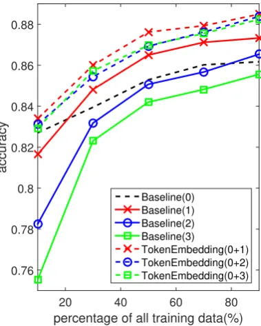
We first train our baseline tagger without the bi-nary feature vector using different amounts of training data and window sizesw ∈ {0,1,2,3}. Figure 3 shows accuracies on the validation set.
percentage of all training data(%)
20 40 60 80
accuracy
0.76 0.78 0.8 0.82 0.84 0.86 0.88
Baseline(0) Baseline(1) Baseline(2) Baseline(3)
TokenEmbedding(0+1) TokenEmbedding(0+2) TokenEmbedding(0+3)
Figure 3: Tagging results. “Baseline(w)” refers to the baseline tagger with context of±wwords; “TokenEmbedding(w+w0)” refers to the token
em-bedding tagger with tagger context of±wwords and token embedding context of±w0 words.
When using only 10% of the training data, the baseline tagger withw= 0performs best. As the amount of training data increases, the larger win-dow sizes begin to outperform w = 0, and with the full training set,w= 1performs best.
Figure3also shows the results of our token em-bedding tagger for w = 0 and w0 ∈ {1,2,3}.5
We see consistent gains when using token embed-dings, higher than the best baseline window for all values ofw0, though the best performance is
ob-tained withw0 = 1. When using small amounts of
data, the baseline accuracy drops when increasing w, but the token embedding tagger is much more robust, always outperforming thew= 0baseline. We then perform experiments using the full training set, showing results in Table 5. For all experiments with the baseline DNN tagger, we fix
5We used focused weighting for the results in Figure 3
usingωj = 2, but found slightly more stable results by
in-creasingωj to 3, still keeping the other weights to 1. Our
val. test (1) Baseline 88.4 88.9 (1) + DNN TE +1.6 +0.9 (2) Baseline + updating 89.4 89.4 (2) + DNN TE +0.6 +0.5 (3) Baseline + features 89.2 89.3 (3) + DNN TE* +0.6 +0.3 (3) + DNN TE +1.2 +1.2 (3) Baseline + features 89.2 89.3 (3) + seq2seq TE* -0.6 -1.0 (3) + seq2seq TE +1.3 +1.0
Table 5: Tagging accuracies (%) on validation (OCT27TEST) and test (DAILY547) sets. Accu-racy deltas are always relative to the respective baseline in each section of the table. “updating” = updates type embeddings during training, “fea-tures” = uses binary feature vector for center word, * = omits center word type embedding.
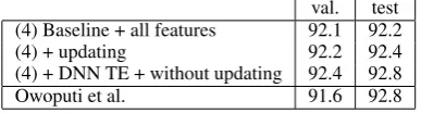
val. test (4) Baseline + all features 92.1 92.2
(4) + updating 92.2 92.4
(4) + DNN TE + without updating 92.4 92.8
Owoputi et al. 91.6 92.8
Table 6: Tagging accuracies (%) on validation (OCT27TEST) and test (DAILY547) sets using all features: Brown clusters, tag dictionaries, name lists, and charactern-grams. Last row is best re-sult from Owoputi et al. (2013).
w = 1; when using token embeddings, we fix w= 0andw0= 1. We also consider updating the
initial word type embeddings during tagger train-ing (“updattrain-ing”) and ustrain-ing the binary feature vec-tor for the center word (“features”).
Using token embeddings consistently outper-forms using type embeddings alone. On the test set, we see gains from token embeddings across all settings, ranging from 0.5 to 1.2. The gains from DNN and seq2seq token embeddings are similar (possibly because we again usew= 0andw0 = 1
for the latter). The baseline taggers improve sub-stantially by updating type embeddings or adding features (settings (2) or (3)), but adding token embeddings still yields additional improvements. When we use token embeddings but remove the type embedding for the word being tagged (de-noted “*”), DNN TEs can still improve over the baseline, though seq2seq TEs yield lower accu-racy. This suggests that the seq2seq TE model is focusing on other information in the window that is not necessarily related to the center word. Comparison to State of the Art. Owoputi et al. (2013) achieve 92.8% on this train/test setup,
us-ing structured prediction and additional features from annotated and curated resources. We add several additional features inspired by theirs. We use features based on their generated Brown clus-ters, namely, binary vectors representing indica-tors for cluster string prefixes of length 2, 4, 6, and 8. We add tag dictionary features constructed from the Wall Street Journal portion of the Penn Tree-bank (Marcus et al.,1993). We use the concate-nation of the binary tag vectors for the three most common tags in the tag dictionary for the word be-ing tagged. We use the 10-dimensional binary fea-ture vector and a binary feafea-ture indicating whether the word begins with a capital letter. All features above are used for the center word as well as one word to the left and one word to the right.
We add several more features only for the word being tagged. We use name list features, adding a binary feature for each name list used byOwoputi et al.(2013), where the feature indicates member-ship on the corresponding name list of the word being tagged. We also include charactern-gram count features forn ∈ {2,3}, adding features for the 3,133 bi/trigrams that appear 3 or more times in the tagging training data.
After adding these features, we increase the hid-den layer size to 2048. We use dropout, using a dropout rate of 0.2 for the input layer and 0.4 for the hidden layers. The other settings remain the same. The results are shown in Table6. Our new baseline tagger improves from 89.2% to 92.1% on validation, and improves further with updating.
We then add DNN token embeddings to this new baseline. When doing so, we set w = 0, as in all earlier experiments. We add two sets of DNN token embedding features to the tagger, one with w0 = 1 and another with w0 = 3. The
re-sults improve by 0.4 over the strongest baseline on the test set, matching the accuracy ofOwoputi et al.(2013). This is notable since they used struc-tured prediction while we use a simple local clas-sifier, enabling fast and maximally-parallelizable test-time inference.
7.2 Dependency Parsing
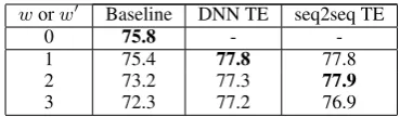
[image:8.595.85.279.290.342.2]worw0 Baseline DNN TE seq2seq TE
0 75.8 -
-1 75.4 77.8 77.8
2 73.2 77.3 77.9
[image:9.595.88.273.61.115.2]3 72.3 77.2 76.9
Table 7: AttachmentF1 (%) on validation set us-ing different models and window sizes. For TE columns, the input does not include any type em-beddings at all, only token emem-beddings. Best re-sult in each column is in boldface.
performance is strong withw0 = 1and 2. When
using token embeddings, we actually found it ben-eficial to drop the center word type embedding from the input, only using it indirectly through the token embedding functions. We use w = −1 to indicate this setting.
The upper part of Table 8 shows the results when we simply use our parsers to output the highest-scoring parents for each word in the test set. Token embeddings are more helpful for this task than type embeddings, improving perfor-mance from 73.0 to 75.8 for DNN token embed-dings and improving to 75.0 for the seq2seq token embeddings.
We also use our head predictors to add a new feature to TweeboParser (Kong et al.,2014). TweeboParser uses a feature on every candidate arc corresponding to the score under a first-order dependency model trained on the Penn Treebank. We add a similar feature corresponding to the arc score under our model from our head predictors. Because TweeboParser results are nondeterminis-tic, presumably due to floating point precision, we train TweeboParser 10 times for both its baseline configuration and all settings using our additional features, using TweeboParser’s default hyperpa-rameters each time. We report means and standard deviations.
The final results are shown in the lower part of Table 8. While adding the feature from the baseline parser hurts performance slightly (80.6→
80.5), adding token embeddings improves perfor-mance. Using the feature from our DNN TE head predictor improves performance to 81.5, establish-ing a new state of the art for Twitter dependency parsing.
8 Conclusion
We have presented a simple and efficient way of learning representations of words in their con-texts using unlabeled data, and have shown how
(1) Baseline parser (w= 0) 73.0 (1) + DNN TE (w=−1, w0= 1) 75.8 (1) + seq2seq TE (w=−1, w0= 1) 75.0 (1) + seq2seq TE (w=−1, w0= 2) 74.2
(2) Kong et al. 80.6±0.25
[image:9.595.316.518.61.155.2](2) + Baseline parser (w= 0) 80.5±0.30 (2) + DNN TE (w=−1, w0= 1) 81.5±0.25 (2) + seq2seq TE (w=−1, w0= 1) 81.0±0.17 (2) + seq2seq TE (w=−1, w0= 2) 80.9±0.33 Table 8: Dependency parsing unlabeled attach-mentF1(%) on test (TEST-NEW) sets for baseline parser and results when augmented with token em-bedding features. Following Kong et al., we report three significant digits.
they can be used to improve syntactic analysis of Twitter. Qualitatively, our token embeddings are shown to encode sense and POS information, grouping together tokens of different types with similar in-context meanings. Quantitatively, us-ing token embeddus-ings in simple predictors con-sistently improves performance, even rivaling the performance of strong structured prediction base-lines. Our code and trained token embedding mod-els are publicly available at the authors’ websites. Future work includes further exploration of token embedding models, unsupervised objectives, and their integration with supervised predictors.
Acknowledgments
We thank the anonymous reviewers, Chris Dyer, and Lingpeng Kong. We also thank the develop-ers of Theano (Theano Development Team,2016) and Lasagne (Dieleman et al., 2015) as well as NVIDIA Corporation for donating GPUs used in this research.
References
Mohit Bansal, Kevin Gimpel, and Karen Livescu. 2014. Tailoring continuous word representations for dependency parsing. InProc. of ACL.
Xinxiong Chen, Zhiyuan Liu, and Maosong Sun. 2014. A unified model for word sense representation and disambiguation. InProc. of EMNLP.
Heeyoul Choi, Kyunghyun Cho, and Yoshua Ben-gio. 2016. Context-dependent word representa-tion for neural machine translarepresenta-tion. arXiv preprint
arXiv:1607.00578.
Ronan Collobert, Jason Weston, L´eon Bottou, Michael Karlen, Koray Kavukcuoglu, and Pavel Kuksa. 2011. Natural language processing (almost) from scratch. Journal of Machine Learning Research12.
Andrew M. Dai and Quoc V. Le. 2015. Semi-supervised sequence learning. InAdvances in NIPS.
Sander Dieleman, Jan Schl¨uter, Colin Raffel, Eben Ol-son, Søren Kaae Sønderby, Daniel Nouri, Daniel Maturana, Martin Thoma, Eric Battenberg, Jack Kelly, et al. 2015. Lasagne: First release.
http://dx.doi.org/10.5281/zenodo.27878.
Felix A. Gers, J¨urgen Schmidhuber, and Fred Cum-mins. 2000. Learning to forget: Continual predic-tion with LSTM. Neural Computation12(10).
Kevin Gimpel, Nathan Schneider, Brendan O’Connor, Dipanjan Das, Daniel Mills, Jacob Eisenstein, Michael Heilman, Dani Yogatama, Jeffrey Flanigan, and Noah A. Smith. 2011. Part-of-speech tagging for Twitter: annotation, features, and experiments.
InProc. of ACL.
Hila Gonen and Yoav Goldberg. 2016. Semi super-vised preposition-sense disambiguation using mul-tilingual data. InProc. of COLING.
Alan Graves, Abdel-rahman Mohamed, and Geoffrey Hinton. 2013. Speech recognition with deep recur-rent neural networks. InProc. of ICASSP.
Jiang Guo, Wanxiang Che, Haifeng Wang, and Ting Liu. 2014. Learning sense-specific word embed-dings by exploiting bilingual resources. InProc. of
COLING.
Sepp Hochreiter and J¨urgen Schmidhuber. 1997. Long short-term memory.Neural Computation9(8).
Eric Huang, Richard Socher, Christopher D. Manning, and Andrew Ng. 2012. Improving word represen-tations via global context and multiple word proto-types. InProc. of ACL.
Sujay Kumar Jauhar, Chris Dyer, and Eduard Hovy. 2015. Ontologically grounded multi-sense represen-tation learning for semantic vector space models. In
Proc. of NAACL-HLT.
Mikael K˚ageb¨ack, Fredrik Johansson, Richard Johans-son, and Devdatt Dubhashi. 2015. Neural context embeddings for automatic discovery of word senses.
InProc. of NAACL-HLT.
Kazuya Kawakami and Chris Dyer. 2015. Learning to represent words in context with multilingual super-vision. InProc. of ICLR Workshop.
Lingpeng Kong, Nathan Schneider, Swabha Swayamdipta, Archna Bhatia, Chris Dyer, and Noah A. Smith. 2014. A dependency parser for tweets. InProc. of EMNLP.
Jiwei Li and Dan Jurafsky. 2015. Do multi-sense em-beddings improve natural language understanding?
InProc. of EMNLP.
Jiwei Li, Thang Luong, and Dan Jurafsky. 2015. A hierarchical neural autoencoder for paragraphs and documents. InProc. of ACL.
Wang Ling, Chris Dyer, Alan W. Black, Isabel Tran-coso, Ramon Fermandez, Silvio Amir, Luis Marujo, and Tiago Luis. 2015. Finding function in form: Compositional character models for open vocabu-lary word representation. InProc. of EMNLP.
Yang Liu, Zhiyuan Liu, Tat-Seng Chua, and Maosong Sun. 2015. Topical word embeddings. In Proc. of
AAAI.
Laurens van der Maaten and Geoffrey Hinton. 2008. Visualizing data using t-SNE. Journal of Machine
Learning Research9.
Mitchell P. Marcus, Mary Ann Marcinkiewicz, and Beatrice Santorini. 1993. Building a large annotated corpus of English: The Penn Treebank.
Computa-tional Linguistics19(2).
Oren Melamud, Jacob Goldberger, and Ido Dagan. 2016. context2vec: Learning generic context em-bedding with bidirectional LSTM. In Proc. of
CoNLL.
Tomas Mikolov, Ilya Sutskever, Kai Chen, Greg S. Cor-rado, and Jeff Dean. 2013. Distributed representa-tions of words and phrases and their compositional-ity. InAdvances in NIPS.
Arvind Neelakantan, Jeevan Shankar, Alexandre Pas-sos, and Andrew McCallum. 2014. Efficient non-parametric estimation of multiple embeddings per word in vector space. InProc. of EMNLP.
Olutobi Owoputi, Brendan O’Connor, Chris Dyer, Kevin Gimpel, Nathan Schneider, and Noah A. Smith. 2013. Improved part-of-speech tagging for online conversational text with word clusters. In
Proc. of NAACL.
Jeffrey Pennington, Richard Socher, and Christo-pher D. Manning. 2014. GloVe: Global vectors for word representation. InProc. of EMNLP.
Matthew E. Peters, Waleed Ammar, Chandra Bhaga-vatula, and Russell Power. 2017. Semi-supervised sequence tagging with bidirectional language mod-els. InProc. of ACL.
Luis Nieto Pi˜na and Richard Johansson. 2015. A sim-ple and efficient method to generate word sense rep-resentations. InProc. of RANLP.
Joseph Reisinger and Raymond J. Mooney. 2010. Multi-prototype vector-space models of word mean-ing. InProc. of NAACL.
Martin Sundermeyer, Ralf Schl¨uter, and Hermann Ney. 2012. LSTM neural networks for language model-ing. InProc. of Interspeech.
Simon ˇSuster, Ivan Titov, and Gertjan van Noord. 2016. Bilingual learning of multi-sense embeddings with discrete autoencoders. InProc. of NAACL.
Ilya Sutskever, Oriol Vinyals, and Quoc V. Le. 2014. Sequence to sequence learning with neural net-works. InAdvances in NIPS.
Theano Development Team. 2016. Theano: A Python framework for fast computation of mathematical ex-pressions. arXiv e-printsabs/1605.02688.
Fei Tian, Hanjun Dai, Jiang Bian, Bin Gao, Rui Zhang, Enhong Chen, and Tie-Yan Liu. 2014. A probabilis-tic model for learning multi-prototype word embed-dings. InProc. of COLING.
Joseph Turian, Lev Ratinov, and Yoshua Bengio. 2010. Word representations: a simple and general method for semisupervised learning. InProc. of ACL. Thuy Vu and D. Stott Parker. 2016. k-embeddings:
Learning conceptual embeddings for words using context. InProc. of NAACL-HLT.
Zhaohui Wu and C. Lee Giles. 2015. Senaware se-mantic analysis: A multi-prototype word represen-tation model using Wikipedia. InProc. of AAAI. Will Y. Zou, Richard Socher, Daniel Cer, and
Christo-pher D. Manning. 2013. Bilingual word embeddings for phrase-based machine translation. In Proc. of