SB@GU at the Complex Word Identification 2018 Shared Task

Proceedings of the Thirteenth Workshop on Innovative Use of NLP for Building Educational Applications, pages 315–321

SB@GU at the Complex Word Identification 2018 Shared Task

David Alfter

Spr˚akbanken University of Gothenburg

Sweden

david.alfter@gu.se

Ildik´o Pil´an

Spr˚akbanken University of Gothenburg

Sweden

ildiko.pilan@gu.se

Abstract

In this paper, we describe our experiments for the Shared Task on Complex Word Iden-tification (CWI) 2018 (Yimam et al., 2018), hosted by the 13th _{Workshop on Innovative}

Use of NLP for Building Educational Appli-cations (BEA) at NAACL 2018. Our sys-tem for English builds on previous work for Swedish concerning the classification of words into proficiency levels. We investigate dif-ferent features for English and compare their usefulness using feature selection methods. For the German, Spanish and French data we use simple systems based on character n-gram models and show that sometimes simple mod-els achieve comparable results to fully feature-engineered systems.

1 Introduction

The task of identifying complex words consists of automatically detecting lexical items that might be hard to understand for a certain audience. Once identified, text simplification systems can substi-tute these complex words by simpler equivalents to increase the comprehensibility (readability) of a text. Readable texts can facilitate information processing for language learners and people with reading difficulties (Vajjala and Meurers, 2014;

Heimann M¨uhlenbock,2013;Yaneva et al.,2016). Building on previous work for classifying Swedish words into different language proficiency levels (Alfter and Volodina,2018), we extend our pipeline with English resources. We explore a large number of features for English based on, among others, length information, parts of speech, word embeddings and language model probabil-ities. In contrast to this feature-engineered ap-proach, we use a word-length and n-gram proba-bility based approach for the German, Spanish and French data.

Our interest for participation in this shared task is connected to the ongoing development of a com-plexity prediction system for Swedish (Alfter and Volodina, 2018). In contrast to this shared task, we perform a five-way classification correspond-ing to the first five levels of the CEFR scale of lan-guage proficiency (Council of Europe,2001). We adapted the pipeline to English, and included some freely available English resources to see how well these would perform on the CWI 2018 task and to gain insights into how we could improve our own system.

2 Data

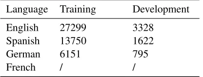
There were four different tracks at the shared task. Table1shows the number of annotated instances per language. For the French sub-task, no training data was provided. Each instance in the English dataset was annotated by 10 native speakers and 10 non-native speakers. For the other languages, 10 annotators (native and non-native speakers) an-notated the data. An item is considered complex if at least one annotator annotates the item as com-plex.

Language Training Development English 27299 3328

Spanish 13750 1622 German 6151 795

French / /

Table 1: Number of instances per language

In the dataset, information about the total num-ber of native and non-native annotators and how many of each category considered a word complex is also available.

A surprising aspect of the 2018 dataset was the presence of multi-word expressions (MWE), which were not part of the 2016 shared task. For

the 2018 task, the training data contains 14% of MWEs while the development data contains 13%.

3 Features

We extract a number of features from each target item, either a single word or a multi-word expres-sion. The features can be grouped into: (i) count and word form based features, (ii) morphological features, (iii) semantic features and (iv) context features. In addition, we use psycholinguistic fea-tures extracted by N-Watch (Davis,2005). In Ta-ble2, we list the complete set of features used for English.

Count features

Length (number of characters) Syllable count (S1)

Contains non-alphanumeric character Is number

Is MWE

Character bigrams (B1)

N-gram probabilities (Wikipedia) In Ogden list

AWL distribution CEFRLex distribution

Morphological features

Part-of-speech Suffix length

Semantic features

Number of synsets Number of hypernyms Number of hyponyms Sense id

Context features

Topic distributions Word embeddings

N-Watch features

British National Corpus frequency (BNC) CELEX frequency (total, written, spoken) In Kuˇcera Francis (KF) list

Sydney Morning Herald frequency (SMH) Reaction time

Bigram frequency (B2) Trigram frequency (T2) Syllable count (S2)

Table 2: Overview of features

Word length in terms of number of characters has been shown to correlate well with complexity in a number of studies (Smith, 1961; Bj¨ornsson,

1968;O’Regan and Jacobs,1992).

Besides the number of characters, we also con-sider the number of syllables (S1 and S2). As the calculation of syllables in English is not straight-forward, we use a lookup-based method for S1. In case the word is not present in the lookup list, we apply a heuristic approach as a fall-back. A high number of multi-syllabic words has been shown to increase the overall complexity of a text (Flesch,

1948;Kincaid et al.,1975), so we assume it could also be helpful in predicting the complexity of smaller units.

The feature related to bigrams (B1) indicates which character bigrams occur in the target item. We calculate all character-level bigrams in the training data and only retain the 36 most predic-tive bigrams using Correlation-based Feature Sub-set Selection (Hall,1999).

N-gram probabilities are based on language models trained on the English Wikipedia dumps from June and July 20151_{. We calculate}

character-level unigram, bigram and trigram probabilities. The Ogden list contains 850 words from Basic English (Ogden, 1944) and this feature indicates whether a word is part of this list.

AWL distribution considers the ten Academic Word List (AWL) sublists (Coxhead,1998) and in-dicates in which lists the word occurs. The AWL list contains word families which appear often in academic texts but excludes general English vo-cabulary, making it specific to the academic con-text. The ten sub-lists are ordered according to fre-quency, so that words from the first sub-list are more frequent than words from the second sub-list, and so forth.

CEFRLex distribution indicates the pres-ence/absence in the 5th_{, 10}th _{and 20}th _percentile

English CEFRLex lists2_{. These lists are obtained}

by aligning and sorting four different vocabulary lists for English (EFLLex) (D¨urlich and Franc¸ois,

2018), French (FLELex) (Franc¸ois et al., 2014), Swedish (SVALex) (Franc¸ois et al., 2016) and Dutch (NT2Lex) (Franc¸ois and Fairon, 2017) by frequency and only taking words which occur in

1_{We already had these pre-calculated language models}

from previous experiments. For simplicity and time rea-sons, we chose not to retrain them on more recent Wikipedia dumps.

the 5th_{, 10}th _{and 20}th _{percentile across all}

lan-guages.

Morphological features include information about parts of speech and suffix length. Suffix length is calculated by stemming the word using the NLTK stemmer (Bird et al., 2009) and sub-stracting the length of the identified stem from the length of the original word.

Semantic features are: number of synsets, num-ber of hyponyms, numnum-ber of hypernyms and sense id. These features are calculated from WordNet (Miller and Fellbaum, 1998). The first three are obtained by calculating how many items WordNet returns for the word in terms of synsets, hyponyms and hypernyms. Sense id is obtained by using the Lesk algorithm (Lesk, 1986) on the sentence the target item occurs in.

Context features consist of topic distribution and word embeddings. For word embeddings, we use the pre-trained Google News dataset embed-dings. We calculate the word context of a wordwi

in a sentenceS∈w1...wnas the sum of word

vec-tors fromw_i−5 towi+5, excluding the vector for

wi. In case there is not enough context, the

avail-able context is used instead. Topic distributions are calculated by first collecting Wikipedia texts about 26 different topics such as animals, arts, ed-ucation or politics. These texts are tokenized and lemmatized. We then exclude words which occur across all topic lists. Topic distribution indicates in which of these topic lists the target item occurs. Features from N-Watch include frequency in-formation from the British National Corpus (BNC), the English part of CELEX, the Kuˇcera and Francis list (KF), the Sydney Morning Herald (SMH); reaction times and bi- and trigram charac-ter frequencies (B2 and T2). While these features are redundant in some case, such as number of syl-lables (S1 and S2), their values can differ due to being calculated differently.

Since our pipeline was not designed to handle multi-word expressions, we address this by a two-pass approach. First, we extract all features for single words and store the resulting vector repre-sentations. Then, for each multi-word expression, if we have feature vectors for all constituents mak-ing up the MWE, we sum the vectors for count-based features such as length and number of sylla-bles and average the vectors for frequency counts. We have experimented with adding all vectors and averaging all vectors, but found that summing

some features and averaging other features not only yields higher scores but also is linguistically more plausible. Context vectors for MWEs are not added but calculated separately as described above with the difference that for a multi-word expres-sion MWE∈wi, ..., wi+koccurring in a sentence

S _∈ w1, ..., wnas the sum of vectors from wi−5

to wi−1 and wi+k+1 to wi+k+5. In case not all

constituents of a multi-word expression have cor-responding vectors from phase 1, we set all feature values to zero and only use the context.

4 Experiments on the English data

We tried three different configurations for the En-glish data set, namely context-free, context-only and context-sensitive. For context-free, we use the features described above, excluding word em-bedding context. For context-only, we only use the word embedding context vectors.For context-sensitive, we concatenate the context-free and context-only features.

4.1 Classification

We tried different classifiers, among others Ran-dom Forest (Breiman,2001), Extra Trees (Geurts et al., 2006), convolutional neural networks and recurrent convolutional neural networks imple-mented in Keras (Chollet et al.,2015) and PyTorch (Paszke et al.,2017). For Random Forest and Ex-tra Trees, we tried different numbers of estimators in the interval[10,2000]and found that generally either 500 or 1000 estimators reached the best re-sults on the development set. For neural networks, we tried different combinations of hyperparame-ters such as the type of layers, number of con-volution filters, adding LSTM layers, varying the number of neurons in each layer. We tried two different architectures, one taking as input the fea-tures extracted as described below and convolving over these features, the other taking both the fea-tures and word embeddings as separate inputs and merging the separate layers before the final layer.

5 Experiments on other languages

5.1 Predicting the German and the Spanish test set

best-performing feature-engineered models at that time (0.81 F1 vs 0.82 F1).

Following this finding, we used character-level n-gram models trained on Wikipedia dumps3 _for

Spanish, German and French and calculated uni-gram, bigram and trigram probabilities for these languages. In addition, we used target item length in characters as additional feature.

5.2 Predicting the French test set

As there was no training or development data for the French test set, we used the n-gram language model to convert each French entry into n-gram probabilities. We then used the n-gram classifiers for English, German and Spanish to predict labels for each word. We tested two configurations:

1. Predict with English, German and Spanish classifier and use majority vote to get the final label

2. Predict with Spanish classifier and use label as final label

The rationale behind the second configuration is that French and Spanish are both Romance lan-guages. The single Spanish classifier might thus model French data better than incorporating also the English and the German classifiers, as German and English are both Germanic languages.

6 Results

Table3shows the results of the best classifiers on both the development data and the test data. For the English News and WikiNews, the best classi-fier is an Extra Trees classiclassi-fier with 1000 estima-tors with the reduced feature set (see subsection

6.1) and trained on each genre separately, as op-posed to the general English classifier trained on all three genres. For all other tasks, the best classi-fier is an Extra Trees classiclassi-fier with 500 estimators with the reduced feature set.

6.1 Feature selection for English

Out of the set of features proposed for a certain task, usually some features are more useful than others. Eliminating redundant features can result not only in simpler models, but it can also im-prove performance (Witten et al.,2011, 308). We

3_{See footnote 1}

F1 (dev) F1 (test) EN News 0.8623 0.8325 EN WikiNews 0.8199 0.8031 EN Wikipedia 0.7666 0.7812 German 0.7668 0.7427 Spanish 0.7261 0.7281

French / 0.6266

Table 3: Results of best classifiers

therefore run feature selection experiments in or-der to identify the best performing subset of fea-tures. We use the SelectFromModel4 _feature

se-lection method as implemented in scikit-learn ( Pe-dregosa et al.,2011). This method selects features based on their importance weights learned by a certain estimator. We base our selection on the development data and the Extra Trees learning al-gorithm, since it performed best with the full set of features. We use the median of importances as threshold for retaining features. For the other pa-rameters, the default values were maintained for the selection.

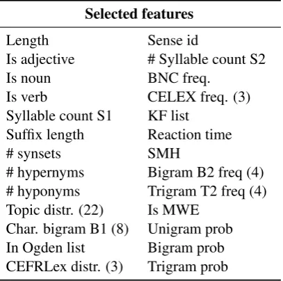
The feature selection method identified a subset of 64 informative features. We list these features in Table4, indicating in parenthesis the amount of features per feature type where it is relevant.

Selected features

Length Sense id

Is adjective # Syllable count S2 Is noun BNC freq.

Is verb CELEX freq. (3) Syllable count S1 KF list

Suffix length Reaction time # synsets SMH

# hypernyms Bigram B2 freq (4) # hyponyms Trigram T2 freq (4) Topic distr. (22) Is MWE

Char. bigram B1 (8) Unigram prob In Ogden list Bigram prob CEFRLex distr. (3) Trigram prob

Table 4: Selected subset of features

The best performing features included, among others, features based on word frequency,

infor-4_{We also tested other feature selection methods, namely}

mation based on words senses and topics as well as language model probabilities.

As only lexical classes were annotated for com-plexity, it is not surprising to see that, even though our pipeline considers all part-of-speech classes, the feature selection picked adjectives, nouns and verbs.

7 Additional experiments on English

7.1 Native vs non-native

Since we had information about how many na-tive speakers and non-nana-tive speakers rated target items as complex, we experimented with training classifiers separately for these two categories of raters. We applied the native-only classifier on the native judgments of the development set, as well as on the non-native judgments, and similarly the native classifier on native judgments and non-native judgments. In all four configurations, we found accuracy to be the same, at about 75%.

7.2 2016 vs 2018

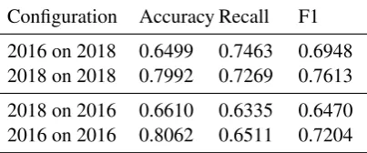
Before this shared task, we experimented with the 2016 CWI shared task data and trained classifiers on it. We tried applying the best-performing clas-sifier trained on the 2016 data on the 2018 devel-opment data, but results were inferior to training on the 2018 training data and predicting 2018 de-velopment data. The same is true in the other di-rection; applying the best-performing 2018 classi-fier on the 2016 data yields inferior results. Table5

shows the result of these experiments. This raises the question of how generalizable these complex word identification systems are and how depen-dent they are on the data, the annotation and the task at hand.

Configuration Accuracy Recall F1 2016 on 2018 0.6499 0.7463 0.6948 2018 on 2018 0.7992 0.7269 0.7613 2018 on 2016 0.6610 0.6335 0.6470 2016 on 2016 0.8062 0.6511 0.7204

Table 5: Results of 2016/2018 comparison

7.3 Genre dependency

During the training phase, we concatenated the English training files for News, WikiNews and Wikipedia into one single training file. We did the same with the development data. We trained

a single, genre-agnostic English classifier on this data. During the submission phase, we used the single classifier but also split the data into the three sub-genres News, WikiNews and Wikipedia again and retrained our systems, which improved perfor-mance. This hints at the genre-dependency of the concept ofcomplexwords.

7.4 Context

As the notion of complexity may be context-dependent, i.e. a word might be perceived as more complex in a certain context, we used word em-bedding context vectors as features. However, our feature selection methods show that these context vectors do not contribute much to the overall clas-sification results. Indeed, of the 300-dimensional word embedding vectors representing word con-text, not a single dimension was selected by our feature selection.

However, if we only look at features which can be derived from isolated words, we also have a problem of contradictory annotations. This means that representing isolated words as vectors can lead to the same vector representation of different instances of a word with different target labels. We calculated the number of contradictions and found that representing each word as a vector leads to 5% of contradictory data points.

8 Discussion

One interesting aspect of the data is the separation of annotators into native and non-native speakers. However, while it can be interesting to try and train separate classifiers for modeling native and non-native perceptions of complexity, and this in-formation can be exploited at training time, us-ing features that rely on the number of native and non-native annotators could not be used on the test data, as the only information given at test time is the total number of native and non-native annota-tors, and these numbers do not vary for the English data.

Our best classifiers are all Extra Trees. All other classifiers that we tested, especially convolu-tional neural networks and recurrent convoluconvolu-tional neural networks, reached lower accuracies. This might be due to insufficient data to train neural networks, a suboptimal choice of hyperparameters or the type of features used.

News, WikiNews and Wikipedia respectively), we reached place 2 on the German data set and place 3 on the French data set. Given the simplicity of the chosen approach, this is slightly surpris-ing. However, we surmise that n-gram proba-bilities implicitly encode frequency among other things, and frequency-based approaches generally perform well.

Further, we found that using only the Spanish classifier on the French data lead to better scores than using all three classifiers and majority vote. This speaks in favor of the hypothesis that closely related languages model each other better. This can be interesting for low-resource languages if there is a related language with more resources.

9 Conclusion

We presented our systems and results of the 2018 shared task on complex word identification. We found that simple n-gram language models per-form similarly well to fully-feature engineered systems for English. Our submission for the non-English tracks were based on this observation, cir-cumventing the need for more language-specific feature engineering.

10 Acknowledgements

We would like to thank our anonymous reviewer for their helpful comments and the organizers of the shared task for the opportunity to work on this problem.

References

David Alfter and Elena Volodina. 2018. Towards Sin-gle Word Lexical Complexity Prediction. In Pro-ceedings of the 13th Workshop on Innovative Use of NLP for Building Educational Applications.

Steven Bird, Ewan Klein, and Edward Loper. 2009.

Natural language processing with Python: analyz-ing text with the natural language toolkit. O’Reilly Media, Inc.

Carl Hugo Bj¨ornsson. 1968.L¨asbarhet. Liber.

Leo Breiman. 2001. Random forests. Machine Learn-ing, 45(1):5–32.

Franc¸ois Chollet et al. 2015. Keras. https:// keras.io.

Council of Europe. 2001. Common European Frame-work of Reference for Languages: Learning, Teach-ing, Assessment. Press Syndicate of the University of Cambridge.

Averil Coxhead. 1998. An academic word list, vol-ume 18. School of Linguistics and Applied Lan-guage Studies.

Colin J Davis. 2005. N-Watch: A program for deriving neighborhood size and other psycholinguistic statis-tics. Behavior research methods, 37(1):65–70.

Luise D¨urlich and Thomas Franc¸ois. 2018. EFLLex: A Graded Lexical Resource for Learners of English as a Foreign Language. In11th International Confer-ence on Language Resources and Evaluation (LREC 2018).

Rudolph Flesch. 1948. A new readability yardstick.

Journal of applied psychology, 32(3):221.

Thomas Franc¸ois and C´edrick Fairon. 2017. Intro-ducing NT2Lex: A Machine-readable CEFR-graded Lexical Resource for Dutch as a Foreign Language.

InComputational Linguistics in the Netherlands 27

(CLIN27).

Thomas Franc¸ois, Nuria Gala, Patrick Watrin, and C´edrick Fairon. 2014. FLELex: a graded lexical re-source for French foreign learners. InLREC, pages 3766–3773. Citeseer.

Thomas Franc¸ois, Elena Volodina, Ildik´o Pil´an, and Ana¨ıs Tack. 2016. SVALex: a CEFR-graded Lex-ical Resource for Swedish Foreign and Second Lan-guage Learners. InLREC.

Pierre Geurts, Damien Ernst, and Louis Wehenkel. 2006.Extremely randomized trees. Machine Learn-ing, 63(1):3–42.

Mark Andrew Hall. 1999. Correlation-based feature selection for machine learning.

Katarina Heimann M¨uhlenbock. 2013. I see what you meanAssessing readability for specific target groups. Data linguistica, (24).

J Peter Kincaid, Robert P Fishburne Jr, Richard L Rogers, and Brad S Chissom. 1975. Derivation of new readability formulas (automated readability in-dex, fog count and flesch reading ease formula) for navy enlisted personnel. Technical report, Naval Technical Training Command Millington TN Re-search Branch.

Michael Lesk. 1986. Automatic sense disambiguation using machine readable dictionaries: how to tell a pine cone from an ice cream cone. InProceedings of the 5th annual international conference on Systems

documentation, pages 24–26. ACM.

George Miller and Christiane Fellbaum. 1998. Word-net: An electronic lexical database.

J Kevin O’Regan and Arthur M Jacobs. 1992. Opti-mal viewing position effect in word recognition: A challenge to current theory. Journal of Experimental

Psychology: Human Perception and Performance,

18(1):185.

Adam Paszke, Sam Gross, Soumith Chintala, Gre-gory Chanan, Edward Yang, Zachary DeVito, Zem-ing Lin, Alban Desmaison, Luca Antiga, and Adam Lerer. 2017. Automatic differentiation in PyTorch.

InNIPS-W.

Fabian Pedregosa, Ga¨el Varoquaux, Alexandre Gram-fort, Vincent Michel, Bertrand Thirion, Olivier Grisel, Mathieu Blondel, Peter Prettenhofer, Ron Weiss, Vincent Dubourg, et al. 2011. Scikit-learn: Machine learning in Python. Journal of Machine

Learning Research, 12(Oct):2825–2830.

Edgar A Smith. 1961. Devereux Readability Index.

The Journal of Educational Research, 54(8):298–

303.

Sowmya Vajjala and Detmar Meurers. 2014. Assess-ing the relative readAssess-ing level of sentence pairs for text simplification. InProceedings of the 14th

Con-ference of the European Chapter of the Association for Computational Linguistics.

Ian H Witten, Eibe Frank, Mark A Hall, and Christo-pher J Pal. 2011. Data Mining: Practical machine

learning tools and techniques. Morgan Kaufmann.

Victoria Yaneva, Irina P Temnikova, and Ruslan Mitkov. 2016. Evaluating the Readability of Text Simplification Output for Readers with Cognitive Disabilities. InLREC.