A Markovian model for reliability and other performance measures of software systems*

by AMRIT L. GOEL and KAZU OKUMOTO Syracuse University

Syracuse, New York

INTRODUCTION

Several studies have been undertaken in recent years to investigate the software failure phenomenon, with the ob-jective of developing analytical models for quantitative as-sessment of software performance. Most of these studies assume that the times between software failures follow an exponential distribution with a failure rate that depends on the number of errors in the system (see, for example, Jelinski and Moranda,5 Littlewood and Verra1l6 _{and Shooman}ll_{). A}

key assumption made in most of these studies is that the errors are removed with certainty when detected. However, as pointed out in Miyamot07 _{and Thayer et al.,l2 errors are} not always corrected when detected. The existing models do not provide a solution for such situations.

In this paper we develop a Markovian model, which we call an Imperfect Debugging Model (IDM), for studying soft-ware failures when ermrs are not removed/corrected with certainty, i.e., for the case of imperfect debugging. Also, expressions are derived for the following probabilistic per-formance measures:

• Time to a completely debugged system. • Time to a specified number of remaining errors. • Number of remaining errors at time t.

• Number of errors detected by time t. • Reliability function.

Actual failure data from a large Department of Defense (DoD) software project are analyzed and the results com-pared with the observed values.

MODEL DEVELOPMENT

The following assumptions are made for developing the model:

1. An error causing a software failure, when detected, is corrected with probability p, while with probability * This work was supported by the Air Force Systems Command's Rome Air Development Center, Griffiss Air Force Base, NY.

q(p

+

q= 1) we fail to completely remove it. Thus, q is the probability of imperfect debugging.

2. The time, Tj to a software failure, when i errors remain in the sysiem, follows an exponential distribution with parameter iA. The parameter A represents the mean error occurrence rate per unit time.

3. The time to remove an error will be neglected in this model.

4. No new errors are introduced during the debugging process.

5. At most, one error is removed at correction time. Let X(t) denote the number of errors remaining in a soft-ware system at time t. We will use this random variable to describe the behavior of the error removal process as a function of time. Further, let N be the number of errors at the beginning of the debugging phase, i.e., X(O)=N.

Suppose that there are i errors in the package at some time. Then from Assumption 1, we note that after the oc-currence of the next failure

X(t)=

{1:-1

w~th probab~l~ty p.

I wlth probabilIty q (1)

In other words, if we were to observe the X(t) process at times of software failures, then its behavior is governed by Equation 1. The transition probabilities Pjj from state i to state j are given by

{ p j=i-l _ q j=i poO-13 1 i= j=O

o

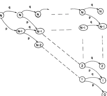
otherwise i, j=O, 1,2, ... , N. (2)

A diagrammatic representation of transitions between states corresponding to Equation 2 is given in Figure 1.

Assumption 2 implies that the Probability Density Func-tion (PDF) and the Cumulative DistribuFunc-tion FuncFunc-tion (CDF) of the random variable Tj are, respectively given by

(3) and

(4)

We note that even though the stochastic process X(I)

770 National Computer Conference, 1979

q q

N-2

Figure I-A diagrammatic representation of transitions between states of X( t).

makes transitions from state to state in accordance with Equation 2, the times spent in various states are random

and are given by Equation 3. Hence, the process {X(t),

t2!::O} forms a semi-Markov process (see, for example, Ross9). A typical realization of this process is shown in

Figure 2. It should be pointed out that in our formulation

the process X(t) undergoes both real and virtual transitions.

This means that after an attempt to remove an error the

state of X(t) may change or may remain unchanged. In

Figure 2, real transitions occur at states N, N - 2 and i while

a virtual transition occurs at state N - 1 .

N N-I

_•

•

N-2 e

-\

(/)

\

w I-~ l-(/)

•

i-I

•

o

_TIME

Figure 2-A typical realization of the X(t) process.

Let

Qjj

(t) denote the one-step transition probability that,

after making a transition into state i, the process X(t) next

makes a transition into state j by time t. In other words, if

a software package has i remaining errors at time zero, then

Q u (t) represents the probability that the next failure,

re-sulting inj remaining errors, will be by time t. Then, we can

show that

Qu(t)=Pu·Fj(t)

for i, j=O, 1,2, . . . , N. Substituting (2) in (5) yields

{ pFi(t) j=i-l Q. (t) = q Fi (1 )

!

= ~ u 1 J=I=O

o

otherwise (5) (6)

For known parameters N, p and X, the probabilities Qu(t)

are obtained from Equation 6. This equation represents the basic model that will be used in the following sections for obtaining the various performance measures for software systems.

EXPRESSIONS FOR PERFORMANCE MEASURES Distribution of time to a completely debugged software

system

Suppose i is the number of errors remaining in a software system at some time during the debugging process and let Gi,o (1) represent the probability that the time required to go

from i to 0 errors is less than or equal to t. In other words,

Gi.O(t) represents the CDF of the time required to get a completely debugged system when the current number of

remaining errors is i.

Recall that at time zero, X(O)= N and at the time of the

first failure

X( )

=

{N -

1 with probability p

t N with probability q (7)

as shown in Figure 1. Suppose that the debugging at the first error occurrence is perfect. Then the probability of going

from N to N-l errors in time [u, u+du] is given by

dQN.N-l (u). If the system clears an error at time u, then the

process X(t) restarts with (N-l) remaining errors at time

u and the probability of going from N - 1 to 0 in time t - u

is GN-1,O(t- u). Hence the probability of going from N to 0

in time t is

f

GN-1,O(t-u)·dQN,N-l(U)=QN,N-l*GN-1,O(t), (8)

where

*

denotes convolution.

Similarly, if the debugging at the first error occurrence is

imperfect, the probability of going from N to 0 in time t is

f

GN,o(t-u)·dQN,N(U)=QN.N*GN,O(t). (9)

Since the events depicted in Equations 8 and 9 are mutually exclusive, we get the renewal equation

In general, we get the renewal equation Gi,o(t)= Qi,i-l* Gi-1,O (t)+ Qi,i* Gi •O (t)

for i= 1, 2, ... , N where Go•o (t)= 1.

(11)

Using the Laplace-Stieltjes (L-S) transform technique (see Ross,9 for example) to solve the renewal Equation 11, we obtain the probability that the software system will be com-pletely debugged by time t as

N

GN.O(t)= ~ CNJ(1-e-,;P~.t). j=l

where

Distribution of time to a specified number of remaining errors

(12)

In many instances a completely debugged software is not cost-effective and we may be willing to tolerate a certain number of remaining errors, say no, which will ensure some desired reliability. The distribution of time to no is then of interest.

Using an approach similar to the one above, we get the renewal equation

G i•no (t)= Qi.i-l* Gi-1,no (t)+ Qi,i* Gi •no (t), (13) for i

=

no

+

1, . . . , N

where Gno>no (t)= 1. Then the probabiliiy that the software system will have no errors by time t, starting with N errors at time 0, is obtained by N-no GN.no(t)= ~ BNJ.no{l-e-(no+j)PAt}, (14) j=l where N' . B _ _ _ '_--:--(_I\i-l_}_

N.i.no=no!}1(N- no-j)! ' no+j'

Distribution of number of remaining errors

Let PN,no (t) represent the probability that there are no errors remaining in a software package at time t, given that there are N errors at the beginning of debugging, i.e.,

PN,no (t)= P{X(t)= no

I

X(O)= N}

which is the so-called state occupancy probability. Condi-tioning on the next failure and fonowing an approach similar to the above, we get the following renewal equations:

Pno,no (t)= e -nOAt + Qno,no* P no.no (t), Nos,N, (15)

no<N. (16)

The· distribution of the number of remaining errors at time t is

PN,no(t)=GN,no(t)-GN,no-dt), no=O, 1,2, . . . ,N (17)

where

G N,N(t)=I, , GN,-l(t)=O.

Finally, the expected number of remaining errors in the software at time t is

N

E[X(t)IX(O)=N]= ~ nOPN,no(t)=Ne-PAt. (18)

no=O

From Equation 18, we note that the number of errors re-maining in the software system is expected to decrease ex-ponentially Qver the debugging time.

Expected number of errors detected by time t

We introduce a new random variable N(t) which denotes the total number of errors detected by time t. The process {N(t), t~O} is called a counting process. We are interested in obtaining the expression for the expected number of er-rors detected, MN (t), during the debugging period, t, when the initial number of errors is N, i.e.

MN (t) = E[N(t)

I

X(O)= N]

which is called a Markov renewal function. By conditioning on the next software failure, we obtain the renewal equations

MJ(t)=Fj(t) + pMj -1

*

Fj(t)

+qMj*Fj(t), j=1,2,.' .. , N where Mo (t)=0. From (19) we obtain

N MN(t)= - (1 - e-PAt ). p 110\ \" .... I (20) By taking the derivative of (20) we can get the error detec-tion rate at time t,

(21) which is exponentially- decreasing over time. This implies that more errors are detected during the early stages of debugging. Note that if we let t~oo we have

which is the expected number of software errors detected by the end of debugging.

Let us now consider the case when the detected errors are separated as new errors and errors which were not corrected due to imperfect debugging. Let N[(t) be a ran-dom variable which denotes the total number of imperfect debugging errors by time t. Then we can show that

772 National Computer Conference, 1979

where

DN(t)=E[N/(t) IX(O)=N].

Note that DN(oo)=q N . Equation 22 implies that 1O<kJ

per-p

cent of the software failures during debugging will be due to imperfect debugging.

Software system reliability

So far we have studied the stochastic behavior of the number of errors in the software system during the debug-ging period. Now we investigate the distribution of the time between software failures and study the problem of reliabil-ity growth. From the second section recall that the random variable Ti denotes the time to next failure when the number of remaining errors is i and Fi(t) is the CDF of Tj • Let Xk

denote the time between the (k - l)st and kth software fail-ures and <l>k(X) be the CDF of X k . Note that X k does depend on the number of remaining errors at the (k-l)st failure but this number is not explicitly known. Further, let

71 k be a random variable which denotes the number of

re-maining errors between the (k-l)st and kth software fail-ures. Then, from the second section we have

711=N <1>1 (x)= F N(X), and <1>2 (X)= pF N-l (x)+qFN(x). In general, we have N <l>k (X)

=

P (Xk.::5 X) =

L

p(Xk::5XI71k=i)p(71k=i) i=N-Ck-ll or k-l <l>k(X)=

I

p[Xk::5XI71k=N-k+ j+ 1)P(71k=N-k+ j+ 1) j=O or <l>k(X)= k-l

I

(k-I)

.

p k-j-l .q FN-Ck-i-ll(X). j j=O J (23) This is called a mixture of exponential distributions with binomial mixing portions. It can be shown that <l>n(x) is a Decreasing Failure Rate (DFR) distribution. The reliability function at the kth stage, i.e., between (k-l)st and kth failure, is given by Rk(x)= p{Xk>x}

=

1-<l>k(X)

- I

_ k-l

.

p q FV-(k-i-ll(X) (k-I) k-j-l j -i=O J where in general F..,(x)

=

1-F .. .{x)= e-'vAX. (24)

From a practical point of view the reliability obtained in (24) is not easy to work with. For computational purposes we use the following approximation.

Rk(x)-e-[N-P<k-OJAX, k= 1,2, . . . (25) For details of this approximation, see Goel and Okumoto.2

APPLICATION TO A LARGE SOFTWARE PROJECT In this section we analyse the error data from a large software project and compute various performance meas-ures using the results of the two preceeding sections. The error data is taken from Fries,l and represents software errors from a large DoD systems development project. The project consisted of approximately 320,090 assembly lan-guage instructions. It included the operational software and the simulation software necessary to develop and test the former. Software Problem Reports (SPRs) were written in the time period from the beginning of configuration manage-ment (approximately start of integration testing) to delivery of the software. A total of 2036 SPRs were encountered during this period and they were categorized into 20 major groups. Data are also included about the source of errors, the type of correction made, and the time to find and fix the error.

For purposes of this analysis, we consider 1612 errors reported during the last 12 months of the software testing phase. For estimating the parameters N, p and A we use the method given in Goel and Okumoto.3 _{The estimated values}

of these parameters are

N=2108, p=0.936 and ~=0.1127.

Substituting

N,

p

and ~ for N, p and A, respectively, in Equation 18, the estimated value of the expected number of remaining errors over the testing period t is obtained as

E[ X( t)

I

X(O)

=

N] =2108e -(.936)(. 1127)t •

A plot of this quantity is shown in Figure 3. Also shown in this figure are the observed values by month. The fitted curves (or MN(t) and DN(t) from Equations 20 and 22 are shown in Figure 4 along with the actual values for these quantities. From Figures 3 and 4 we see that the model seems to describe the behavior of the software error phe-nomenon very well.

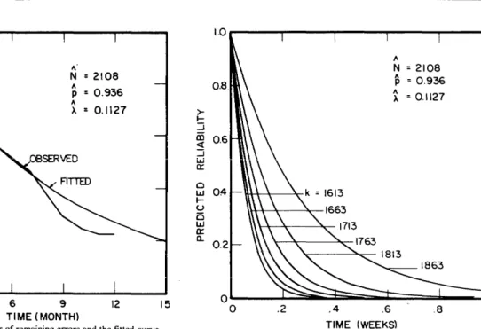
The reliability function for the system is obtained from Equation 25 as

Rk(x)= e -[21OS-.936(k-1)](01l27)x.

Plots of reliability for k=1613(50)1863, i.e., for the cases when the number of errors removed is 1612(50)1862, are shown in Figure 5. From these plots the extent of reliability growth with k can be easily evaluated. For example,

R 1613 (0.1)=0.24 while _{R 1863 (0.1)=0.74,} i.e., the value of

R(O.I) increases by 200 percent when k goes from 1613 to 1863.

The plots in Figure 5 can also be used to determine the expected time required to achieve a desired reliability. Sup-pose our objective is to have a reliability of 0.3 at 0.2 weeks.

2200~----~----~----~~----~----~

'"

N = 2108 A P

=

0.936 1760 (/) A. A

=

0.1127 a:: 0 a:: a:: LLI ₁₃₂₀ ~ Z <i ~ 800 LLI a:: u... 0 a:: LLI m 440 ~ :;) z 0 0 3 6 9 12 15 TIME (MONTH)

Figure 3-Plots of the number of remaining errors and the fitted curve.

We want to know the number of errors that must be removed to achieve this reliability. In other words we want to know

the value of k that yields Rk(0.2)=0.3. From Figure 5, we

see that R 1813(0.2)=0.3 so that k= 1813 errors to achieve

desired reliability for the software system. Then the number of remaining errors will be

or 1800 (/)

~

a:: LLI ~ 900 "-(f) IL.

o

a:: 600 LU

i

:l Z

"

N

"

p

"

A 110=2108- .936(1813-1) 110=412. =2108 =0.936 = 0.1127 3 IMPERFECT DEElJGGING (FITTEDlJl

r

ACTUALl \ 6 9 12 nME(MONTHl

Figure 4-Total and imperfect debugging errors by month.

15 1.0 0.8 >- I-:J CD _0.6 <[ :J w a:: o LLI 04 I-u

o

LLI a:: a.. 0.2

,.

N

=

2108

"

=

0.936 P 1\

=

0.1127 A OL---~~~~=-~~~:=~----J

o

.2 .4 .6 .8 1.0 TIME (WEEKS)

Figure 5-Plots of the reliability function for various values of k.

The expected time required to remove (N - no) errors is

1 N I l N-l

I-LN,no= \

L -:

= \ In - - 1 .

P"-j=no+1 J p,,- no

+

For our case, we get

1 2108+ 1

,u2108.412 = (0.936)(0.1127) ·In 412+ 1 = 15.46 months . . In other words, to achieve the desired reliability, we will

need to continue testing for 15.46-12=3.46 additional

months. CONCLUSION

We have developed an imperfect debugging model (IDM) for software systems and derived expressions for various performance measures in terms of the first passage time distribution of the underlying semi-Markov process. The failure data from a large software project were analyzed using the model developed in this paper. A comparison of the fitted and the obseived values indicates that the model provides a good description of the underlying failure phe-nomenon. Also, reliability curves were used to determine the debugging time required to achieve a desired level of software system performance.

REFERENCES

1. Fries, M. J., "Software Error Data Acquisition," Boeing Aerospace Co., Final Technical Report, RADC-TR-77-130, IfJ"77.

2. Goel, A. L., and K. Okumoto, "An Imperfect Debugging Model for Reliability and Other Quantitative Measures of Software Systems," RADC-TR-155, Vol. I, 1978.

774 National Computer Conference, 1979

3. Goel, A. L., and K. Okumoto, "An Analysis of Recurrent Software Errors in a Real-Time Control System," Proc. of ACM, 1978, pp. 496-501.

4. Goel, A. L., and K. Okumoto, "A Time-Dependent Error Detection Rate Model for Software Reliability and Other Performance Measures," (to appear) IEEE Trans. Rei. (Special issue on Software Reliability), 1979. 5. Jelinski, Z., and P. Moranda, "Software Reliability Research,"

Statisti-cal Computer Performance Evaluation, W. Freiberger (ed.), Academic Press, 1972, pp. 465-484.

6. Littlewood, B., and J. L. Verrall, "A Bayesian Reliability Growth Model for Computer Software," Applied Statistics, Vol. 22, 1973, pp. 332-346. 7. Miyamoto, I., "Software Reliability in On-Line Real Time Environ-ment:' Proc. 1975 International Conference on Reliable Software. pp. 194-203.

8. Okumoto, K., and A. L. Goel, "Availability and Other Performance Measures of Software Systems Under Imperfect Maintenance," Proc. of Computer Software & Applications Conference, 1978, pp. 35-40. 9. Ross, S. M.,Applied Probability Models with Optimization Applications,

Holden-Day.

10. Schneidewind, N. J., "Analysis of Error Processes in Computer Soft-ware," Proc. 1975 International Conference on Reliable Software. pp. 337-346.

II. Shooman, M. L., "Operational Testing and Software Reliability Esti-mation During Program Development," Record 1973 IEEE Symposium on Computer Software Reliability, pp. 51-57.

12. Thayer, T. A., M. Lipow and E. C. Nelson, "Software Reliability Study," TRW Defense & Space Systems Group, Final Technical Report, RADC-TR-76-238. 1976.