Decomposition and duality based approaches to stochastic integer programming

(1)

Decomposition and duality based approaches to Stochastic

Integer Programming

A thesis submitted in fulfilment of the requirements

for the degree of Doctor of Philosophy

Jeffrey Christiansen

BSc Adv. Hons., Monash University

School of Science

College of Science, Engineering and Health

RMIT University

(2)

Declaration

I certify that except where due acknowledgement has been made, the work is that of the author alone; the work has not been submitted previously, in whole or in part, to qualify for any other academic award; the content of the thesis is the result of work which has been carried out since the official commencement date of the approved research program; any editorial work, paid or unpaid, carried out by a third party is acknowledged; and, ethics procedures and guidelines have been followed.

I acknowledge the support I have received for my research through the provision of an Australian Government Research Training Program Scholarship.

Jeffrey Christiansen June 21, 2018

(3)

Acknowledgements

First and foremost, I would like to thank my supervisors Andrew Eberhard (whose door always seems to be open) and Natashia Boland (who battled through various inconveniences and injuries) for their excellent guidance and steadfast support. For the same reasons, my heartfelt thanks to Brian Dandurand, who acted as my unofficial third supervisor (despite this appearing nowhere in his job description). I couldn’t have asked for a better team.

The research contained in this thesis has been carried out within a larger collaborative research project. Besides Andrew, Natashia and Brian, the other members of this project were Fabricio Oliveira and Jeff Linderoth, both of whom made substantial contributions to both our research and my education as a researcher. James Luedtke joined forces with us for our first paper and also merits mention here. The contributions made to the research in this thesis by the aforementioned collaborators is documented in the Preface on the following page.

Thanks are also due to the friendly support staff at the National Computational Infrastruc-ture (NCI) and the (unfortunately now retired) V3 Alliance (VPAC) for their technical assistance. Without their trouble-shooting expertise the experimental component of this research would have taken much longer, in terms of both implementation and execution.

Finally, I’m very grateful to my family, friends and colleagues for their encouragement and support. I expect to speak with many of you personally, but in particular I’d like to thank the various people I’ve lived with over the last four years for their understanding when deadlines became pressing, the RMIT Optimisation group for broadening my horizons (particularly Vera Roshchina, who organised the group for several years), and my office companions and fellow travellers on the PhD track for always being ready to have a laugh.

(4)

Preface

Some of the material in this thesis is based on published multi-author papers.

• Chapter 4 is based on [16]. The other co-authors of this paper are Natashia Boland, Brian Dandurand, Andrew Eberhard, Jeff Linderoth, James Luedtke and Fabricio Oliveira.

• Chapter 5 is based on [17]. The other co-authors of this paper are Brian Dandurand, Fabricio Oliveira, Andrew Eberhard and Natashia Boland.

• Chapter 6 is based on [93]. The other co-authors of this paper are Fabricio Oliveira, Brian Dandurand and Andrew Eberhard.

From these sections and chapters, the experimental results in Sections 4.3 and 5.3 and the theoretical results developed in Section 6.2 were completed by Jeffrey Christiansen. The remainder of these chapters is the result of equal collaboration between the authors of each respective paper. The work in the chapters not previously listed was also completed by Jeffrey Christiansen.

(5)

List of Figures

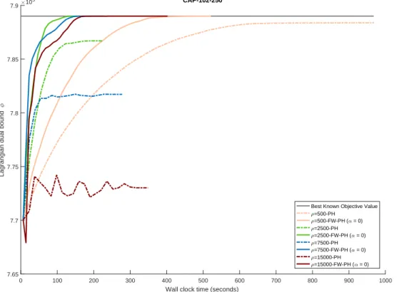
4.1 PH and FW-PH convergence profiles for CAP-101-250 (α0) . . . 81

4.2 PH and FW-PH convergence profiles for CAP-101-250 (α0) . . . 81

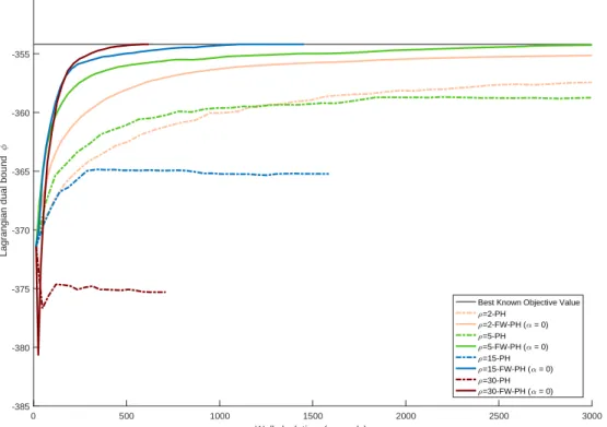
4.3 PH and FW-PH convergence profiles for DCAP-233-500 (α 0) . . . 82

4.4 PH and FW-PH convergence profiles for DCAP-233-500 (α 0) . . . 82

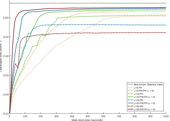
4.5 PH and FW-PH convergence profiles for SSLP-5-25-50 (α0) . . . 83

4.6 PH and FW-PH convergence profiles for SSLP-5-25-50 (α0) . . . 83

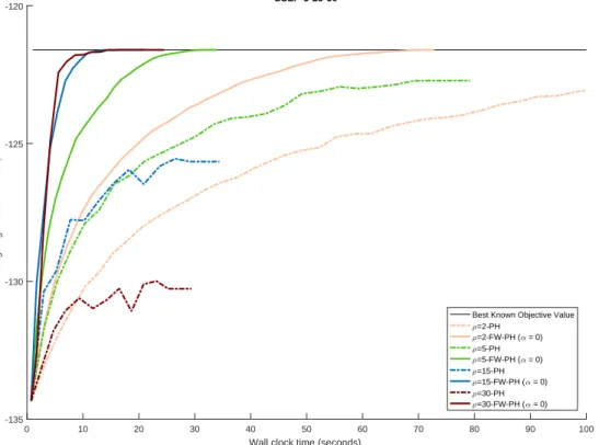
4.7 PH and FW-PH convergence profiles for for SSLP-10-50-100 (α0) . . . 84

4.8 PH and FW-PH convergence profiles for for SSLP-10-50-100 (α0) . . . 84

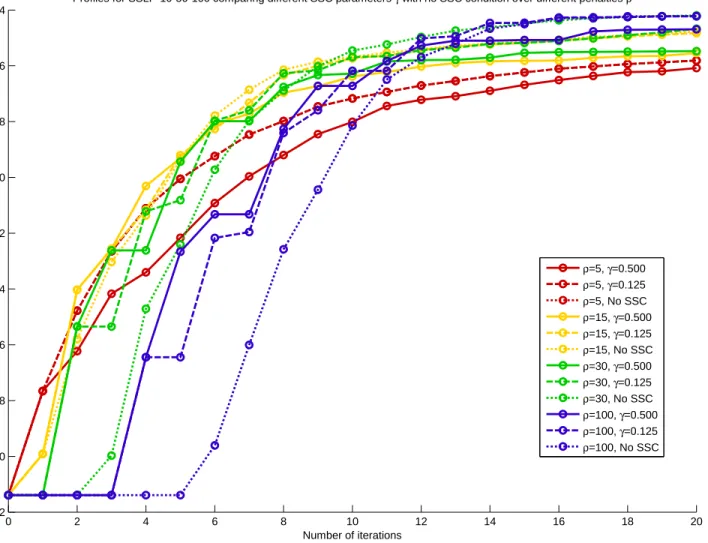
5.1 Applying SDM-GS-ALM to DCAP-233-500 using different penalties and parameter-izations for the serious step condition . . . 118

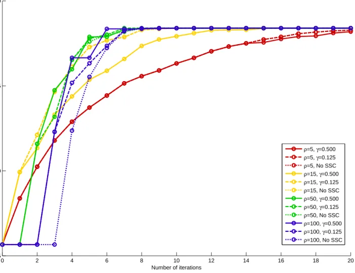
5.2 Applying SDM-GS-ALM to CAP-101-250 using different penalties and parameteri-zations for the serious step condition . . . 119

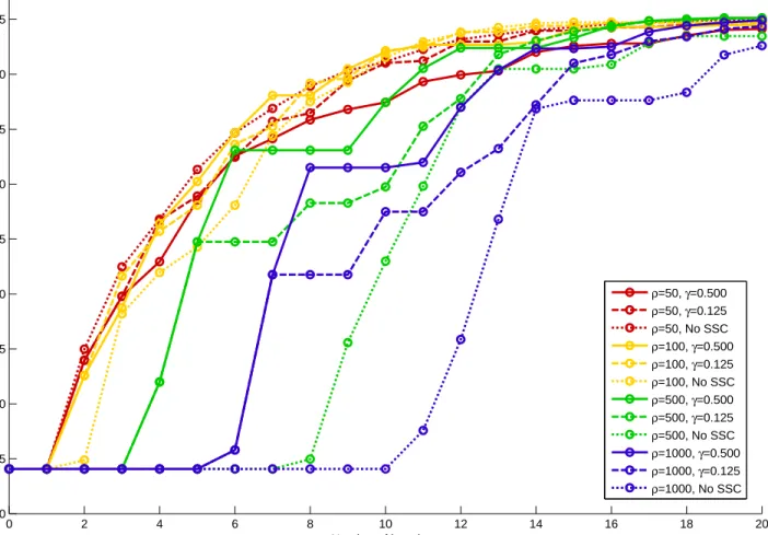
5.3 Applying SDM-GS-ALM to SSLP-5-25-50 using different penalties and parameteri-zations for the serious step condition . . . 120

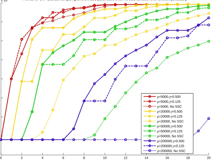
5.4 Applying SDM-GS-ALM to SSLP-10-50-100 using different penalties and parameter-izations for the serious step condition . . . 121

6.1 PBGS results for CAP instances . . . 153

6.2 PBGS results for DCAP instances . . . 153

6.3 PBGS results for SSLP instances . . . 154

(10)

List of Tables

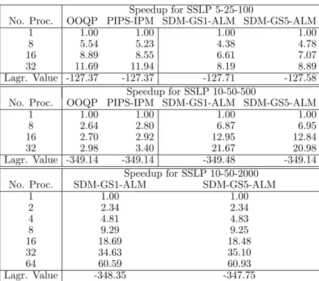
4.1 FW-PH result summary for CAP problem instances: dual bounds. . . 77 4.2 FW-PH result summary for DCAP problem instances: dual bounds. . . 78 4.3 FW-PH result summary for SSLP problem instances : dual bounds. . . 79 5.1 Comparing speedup and final best Lagrangian bound of SDM-GS-ALM, OOQP and

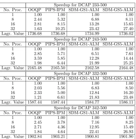
PIPS-IPM for SSLP instances . . . 124 5.2 Comparing speedup and final best Lagrangian bound of SDM-GS-ALM, OOQP and

PIPS-IPM for DCAP instances . . . 125 5.3 Comparing iteration count and runtime of SDM-GS-ALM, OOQP and PIPS-IPM for

SSLP instances . . . 125 5.4 Comparing iteration count and runtime of SDM-GS-ALM, OOQP and PIPS-IPM for

DCAP instances . . . 126

(11)

Abstract

Stochastic Integer Programming is a variant of Linear Programming which incorporates integer and stochastic properties (i.e. some variables are discrete, and some properties of the problem are randomly determined after the first-stage decision). A Stochastic Integer Program may be rewritten as an equivalent Integer Program with a characteristic structure, but is often too large to effectively solve directly. In this thesis we develop new algorithms which exploit convex duality and scenario-wise decomposition of the equivalent Integer Program to find better dual bounds and faster optimal solutions. A major attraction of this approach is that these algorithms will be amenable to parallel computation.

(12)

Chapter 1 Introduction

Optimisation is a field of mathematics which provides tools for making optimal decisions in a given situation. Decision problems are classified by how they can be mathematically represented. This classification determines which algorithms can be effectively and efficiently applied to any given problem.

A powerful modelling technique in optimisation is Linear Programming, which allows us to solve decision problems which can be represented as Linear Programs. A Linear Program consists of a linear objective function which must be minimised or maximised subject to a set of linear constraints. We can represent a generic linear program with n decision variables and m linear inequality constraints in the following form:

ζLP min x c1x1 cnxn s.t.a1,1x1 a1,nxn¤b1 .. . am,1x1 am,nxn ¤bm (1.1)

To abbreviate this formulation, define

x: x1 .. . xn , c: c1 .. . cn , and b : b1 .. . bm

as the vectors of decision variables, objective coefficients and linear constraint constants respectively, and A: a1,1 a1,2 . . . a1,n a2,1 a2,2 . . . a2,n .. . ... . .. ... am,1 am,2 . . . am,n 2

(13)

3 as the matrix of linear constraint coefficients. We can now represent (1.1) using matrix algebra in the condensed form:

ζLP min

x c T_x

s.t.Ax¤b

(1.2) We will use similar abbreviations when formulating optimisation problems in subsequent chapters. In fact, since additional indices to distinguish variable vectors will frequently be required, from this point onward the notationxi will not denote theith variable in the vectorxunless this is specifically

indicated in the text.

Linear Programming is a valuable tool for modelling decision problems but has several limita-tions. We will focus on two of these limitalimita-tions. First, a Linear Program cannot model discrete decisions (such as a yes/no decision); all decision variables in a Linear Program must be continuous. Second, a Linear Program cannot model a problem in which some of the problem data is unavailable when the first decision needs to be made. Discrete decisions and imperfect knowledge are common properties of real-life decision problems, and a more general framework than Linear Programming is necessary to model these problems accurately.

Stochastic Mixed-Integer Linear Programming, typically shortened to Stochastic Integer Pro-gramming, generalises the concept of Linear Programs to account for these limitations. Incorporat-ing binary and integer variables into a standard Linear Program formulation is a straightforward process, although solving the resulting non-convex optimisation problem is frequently difficult. On the other hand, there are several valid approaches to incorporating a stochastic element into a Lin-ear Program so that the initial decisions must be made in conditions of uncertainty. The resLin-earch in this thesis focuses on a scenario-based approach in which initial decisions must be made before the outcome scenario is known, then recourse decisions are made in reaction to the outcome scenario.

A well-known algorithm for solving scenario-based Stochastic Programming problems is the Progressive Hedging algorithm of Rockafellar and Wets [98]. This algorithm calculates what the best initial decision would be if the outcome scenario were known beforehand (for each possible outcome scenario), then tries to find an intermediate solution which is reasonable for all outcome scenarios by alternately updating the decision variables, a set of averaged consensus variables, and the dual multipliers.

(14)

in that it is guaranteed to converge to the global optimal solution. The algorithm may also be applied to Stochastic Integer Programs but the guarantee of optimal convergence does not apply; since the averaging operation is not well defined on an integer set this outcome is not surprising.

The main contributions of this thesis fall into two major classes. First, we will define algorithms for Stochastic Integer Programming which improve on Progressive Hedging and more generally the state of the art in Stochastic Integer Programming, either in the direction of calculating dual bounds or in finding high-quality feasible solutions. These algorithms are based on a similar alternating-update framework, but with structures and goals that are better suited to an integer programming environment. Second, we will explore the underlying theory which motivates and justifies the construction of these algorithms.

The main chapters of this thesis are structured as follows.

Chapter 2 formalises and elaborates on the background material presented in the Introduction. This chapter also contains a review of the current literature in stochastic integer optimisation and related fields of mathematics.

Chapter 3 describes the Frank-Wolfe method, several of its generalisations, and their appli-cations. Section 3.2 extends existing knowledge by demonstrating that these Frank-Wolfe-type methods can be applied to solving the convex hull relaxation of integer programs. This technique is employed in Chapters 4 and 5. Section 3.3 demonstrates that the Frank-Wolfe method can be applied to non-smooth optimisation problems.

Chapters 4 and 5 use a modified version of the Progressive Hedging algorithm to compute the ordinary Lagrangian dual bound of a Stochastic Integer Program directly. The primary algorithmic difficulty in this approach is in solving subproblems over the convex hull of the feasible set. The main results of Chapters 4 and 5 are included in the published papers [16] and [17] respectively.

Chapter 6 takes the alternate approach of constructing penalty functions which result in strong augmented Lagrangian duality. The primary algorithmic difficulty in this approach is in dealing with the restrictions which this places on the penalty function (in particular, non-differentiability). Having done this, an alternating update algorithm is used to obtain high-quality primal feasible solutions. The main results of Chapter 6 are included in the published paper [93].

Chapter 7 proposes an modified version of the algorithm developed in Chapter 6 which has stronger theoretical properties when applied to a Stochastic Mixed-Integer Program with only

(15)

in-5 teger variables in the first stage.

Chapter 8 summarises and concludes the results presented in the thesis and outlines potential directions for future research.

(16)

Chapter 2 Background and Literature Review

2.1 Introduction

2.1.1 Integer Linear Programming

AMixed Integer Linear Program(MILP), typically abbreviated toMixed Integer Program (MIP) or Integer Program(IP), may be written in the following general form:

ζIP mincTx

s.t.Ax ¤b x¥0

xP _Rnq_Zq

(2.1)

This MIP has n decision variables, represented by the vector x. n q of these variables are continuous, and the remainingq are discrete or integer variables. The vectorchas the same length asxand defines the coefficients for each variable in the linear objective function. Ais a lnmatrix and b is a vector of length l, which together define the constraints on the decisions variables as a set ofl inequalities.

A particular choice of decision variables x is called a solution. If a solution satisfies all of the conditions of the problem, then it is a feasible solution. If a feasible solution yields the best possible objective value across all feasible solutions, then it is an optimal solution. In this case the objective is being minimised, so the best possible objective value is the smallest.

Equation (2.1) may appear restrictive since it does not account for differences in objective and constraint type, or for different variable bounds. However, it is possible to reformulate any

(17)

7 integer linear program with equalities, negative variables, or a maximisation objective in the form of Equation (2.1), and so any results proved for Equation (2.1) may be generalised to other forms. In practice it is often more intuitive to construct a MIP using a combination of equalities and inequalities, and with a variety of variable bounds.

2.1.2 Stochastic Programming

The representation of a problem as a MIP assumes that all decisions may be made in advance with full knowledge of what effect they will have. Unfortunately this is not always the case. In many practical problems it is necessary to make decisions before everything about the problem is known with certainty. For example, when scheduling train networks the exact number of passengers each day and the occurrence of any mechanical faults are not known with certainty when the timetable is arranged. In agriculture, the weather conditions which will occur in a particular year are not known when the crops are planted.

In both of these examples and in many other practical problems the future conditions are not known with certainty. It is possible to model this uncertainty with a probability distribution. For example, the probability distributions associated with the set of outcomes corresponding, for example, to high or low passenger traffic, good or bad weather, and the frequency of mechanical faults may be estimated using previous data, which allows a partially informed decision to be made. Different possible outcomes are modelled as separate scenarios, each of which is assigned a probability of occurring. Stochastic programs aim to find the decision which has the best average outcome across all scenarios.

There are some problems which arise when applying the answer obtained by solving a stochastic program to the real world. First, the assignment of probabilities to outcome scenarios is often made without knowledge of the exact actual probabilities of all outcomes; an informed guess must be made. Second, it may not be practical to examine all possible outcome scenarios; the number of outcome scenarios may be prohibitively large, or infinite in the case of a continuous random distribution. This second problem is addressed by taking a representative sample of the set of possible outcomes as the scenario space for the purposes of obtaining a tractable stochastic program.

These issues mean that the optimal solution of a stochastic program will not necessarily be ex-actly “optimal” in the real world. Therefore, algorithms for stochastic programs frequently prioritise

(18)

finding a “good” solution quickly over finding an “optimal” solution.

The work presented herein will generally employ a decision stage based approach to modelling the stochastic elements of a given problem. These models may have two or more stages. A decision problem with two stages will be referred to as a two-stage stochastic program. A problem with more than two decision stages will be referred to as a multi-stage stochastic program.

In a two-stage stochastic program, the first stage decisions or initial decisions are made before the outcome scenario is known. After the outcome scenario is determined, thesecond stage decisionsorrecourse decisions can be made. For example, in the hypothetical train scheduling problem above, if a mechanical fault occurs it may be possible to reschedule other trains to cover the gap.

A multi-stage stochastic program is structured similarly. However, instead of fully unveiling the final outcome scenario in a single step, it is revealed in several discrete steps. Recourse decisions may be made at each of these steps. The structure of the outcome scenarios is typically represented with a tree structure.

An alternative approach to modelling stochastic aspects of a problem is chance-constrained programming. In a chance-constrained program, one or more constraints must be satisfied with a given probability (or degree of certainty). A chance constraint may be written in the form

P pfpxq ¤bq ¥p,

which has the meaning “xmust be chosen such that the probability that the constraint fpxq ¤ b is satisfied is greater than or equal top”.

Chance constraints are more appropriate to some classes of problems than the two- or multi-stage approach, and can more directly tackle problems involving continuous random distributions.

Chance-constrained programming is outside the scope of this project. More detail about this approach may be found in, e.g. [84].

2.1.3 Stochastic Programming Formulation

Two-stage stochastic programs have a much simpler structure than multi-stage stochastic programs. For the purposes of simplicity and clarity, the following introductory explanation of decision-stage based Stochastic Program problem formulation will focus on the two-stage case.

(19)

9 Two-stage stochastic programs are modelled with two sets of variables, corresponding to the first-stage and second-first-stage decisions. Since the first-first-stage decisions must be made before determination of the random variable, there is a single set of first-stage variables across all possible scenarios. Since the second-stage decisions may be made after the random outcome is observed, and may therefore respond to it, there are different sets of second-stage variables for each scenario.

A Two-stage Stochastic Mixed Integer Linear Program (SMILP), abbreviated here to Stochastic Integer Program(SIP), may be written in the following general form:

ζSIP min x c T_x ¸ sPS psrQpx, sqs s.t.Ax ¤b x¥0 xP _Rnq_Zq (2.2) where Qpx, sq min y d T sy s.t.Wsy ¤hsTsx y¥0 yP _Rmr_Zr (2.3)

In an SIP, the second-stage problem for each possible scenario is modelled as a MIP, with the first-stage decision used as a parameter. The expected value of the second-stage problem across all scenarios is added to the first-stage problem as a penalty or incentive in the objective function.

The set S is the set of all possible outcome scenarios s. The expected value of the second-stage problem, given a first second-stage decision, is found by taking the average value of the second-second-stage decision problem across all possible scenariossPS, weighted by the probabilityps of each scenario

s. We will always assume that °_s_P_Sps 1.

This IP has n first-stage decision variables, represented by the vector x, and m second-stage decision variables, represented by the vector y. A full solution to the two-stage SIP consists of a single first-stage decision and multiple second-stage decisions, each of which corresponds to an outcome scenario. A particular choice of decision variables for each stage and outcome scenario is sometimes referred to as a policy. This term is used because we cannot make all of the decisions required in the problem which the stochastic program represents at a single point in time, but we

(20)

can initially define a policy which chooses decisions when and as appropriate. To be feasible a policy must satisfy all constraints on both the first- and second-stage variables.

In the context of SIP formulations such as (2.2) our problem data is represented as follows. cand

dare vectors of length n and m respectively which define the objective functions for the first-stage and second-stage problems. A is a matrix and b is a vector which together define the first-stage constraints Ax ¤ b. As the second-stage decision y has not yet been made in the first stage, the first-stage constraints do not refer to those decision variables. SimilarlyWsand Tsare matrices and

hs is a vector which together define the second-stage constraints Wsy¤hsTsx for each scenario

s. Within the Qpx, sqsubproblem the first-stage decision has already been made and is treated as a constant, so theTsx term is written on the right-hand side of the second-stage constraints in this

formulation.

This formulation does not give any explicit guarantees that the second-stage problems Qpx, sq

will be bounded or feasible for all possible first-stage decisions x. To correct this we may enforce an additional recourse condition. ζSIP _{as defined in (2.2) and (2.3) has} _{relatively complete}

recourse if Qpx, sq 8 for all x which satisfy the first-stage constraints Ax¤ b and x¥ 0. The stronger condition of complete recourse holds if Wsy¤z for all scenarios s and vectorsz of real

numbers with the appropriate dimension.

The formulation given in (2.2) for ζSIP _{has the disadvantage that most of the complexity is}

concealed within the Qpx, sq function. To address this problem, ζSIP _{can be reformulated as a}

singledeterministic equivalent MIP as follows:

ζSIP min x,y1,...,y|S| cTx ¸ sPS ps dT_sys s.t.Ax¤b Tsx Wsys¤hs @sPS x¥0, y ¥0 xP_Rnq_Zq yP _Rmr_Zr (2.4)

This is an ordinary MIP and in principle may be solved using techniques for solving ordinary mixed integer programs. For real world problems, since there is a separate set of variables and constraints for each scenario, the MIP is invariably very large and therefore exceptionally difficult to solve in

(21)

11 this way.

However, this MIP does have a particular structure imposed by its origins as an SIP, which allows specialised algorithms to solve it much more easily. The principle behind these algorithms is to separate, or decompose, the problem into smaller subproblems.

Algorithms based onstage-wise decomposition, alternately namedprimal decomposition, separate the variables and constraints based on which decision stage they correspond to. The L-shaped method (see e.g. [71]) is a standard stage-wise decomposition method. Stage-wise decompo-sition methods, like Benders decompodecompo-sition, are often strongly based on duality and are thus open to further development with the application of new duality methods for Integer Programming, but are less well adapted to parallel decomposition.

Algorithms based on scenario-wise decomposition, alternately named dual decomposi-tion, separate the variables and constraints based on which outcome scenario they correspond to. Lagrangian duality gives a theoretical basis for scenario-wise decomposition on which many algo-rithms have been constructed. Since there are a large number of scenarios in an SIP, and the subproblems corresponding to each scenario are not strongly dependent on each other, scenario-wise decomposition offers a great deal of scope for parallel computation. As such, scenario-scenario-wise decomposition methods will be a primary focus of this research.

2.1.4 Introduction to Lagrangian Duality

In some constrained optimisation problems, a particular subset of the constraints make the prob-lem significantly more difficult to solve. Conversely, if these constraints could be removed from the problem it would be easier to solve. These constraints generally provide important information about the problem, so simply ignoring them is not practical and will not result in a useful answer. However, it is possible to move this information from the constraint into the objective using La-grangian duality.

Consider a general MIP of the form:

ζIP min x c T x s.t.Qxr xPX (2.5)

(22)

where the term x P X represents the “easy” constraints as well as bounds and integrality of the variables. For the purposes of this discussion thesconstraints represented byQxrare considered difficult constraints. In the context of duality, thex variables are referred to asprimal variables.

The Lagrangian corresponding to ζIP _is:

Lpx, λq cTx λTpQxrq (2.6) The corresponding Lagrangian dual functionis

ζLRpλq min

x Lpx, λq

s.t.xP X

(2.7) and the corresponding Lagrangian dual problemis

ζLD max

λ ζ

LR_p_λ_q _(2.8)

The vector λ of dual variables has length s. In the case where x consists of only continuous variables, the initial program is convex and the Lagrangian dual is a strong dual, meaning that

ζLD _ζIP _{(e.g. [100, Theorem 3.27]).}

Ifxcontains integer variables the problem is no longer convex, and a duality gapbetween ζIP

and ζLD _{may occur.} _ζLD _{is still guaranteed to be a} _{weak dual} _to _ζIP _{— it yields a lower bound}

on the value ofζIP_{, which provides information and may contribute to finding the solution for} _ζIP

via another method such as Branch-and-Bound.

Definition 2.1 Given a set X, The convex hull of X, denoted convpXq, is the smallest convex

set containing X. A constructive definition will be given in Section 2.3.2.

A primal characterisation of the Lagrangian dual problem is

ζLD min x c T_x s.t.Qxr xP convpXq (2.9)

(see e.g. [46]). This is a primal problem which has the same optimal value as the Lagrangian dual problem. Furthermore it is a continuous programming problem, as taking the convex hull of the

(23)

13 feasible setX removes the integer restriction on the decision variables. In practice it is challenging to calculate convpXq and model it with linear constraints.

The augmented Lagrangian corresponding to ζIP _is:

Lρpx, λq cTx λTpQxrq ψρpQxrq (2.10)

The corresponding augmented Lagrangian dual function is

ζ_ρLR pλq min

x Lρpx, λq

s.t.xPX

(2.11) and the corresponding augmented Lagrangian dual problem is

ζ_ρLD max

λ ζ LR

ρ pλq (2.12)

The augmenting term ψρp_Qx_rq _{is intended to penalise decisions which violate the difficult}

con-straints Qx r. The augmenting function ψρpq has the properties ψρp0q 0 and ψρpuq ¡ 0 for all u 0, and determines the character of the penalty for violation of the hard constraints. The penalty parameter ρ is a strictly positive scalar parameter which determines the size of the penalty. The typical augmenting function used in most applications of augmented Lagrangian duality is:

ψρpuq ρ 2}u}

2

2 (2.13)

Similarly to the ordinary Lagrangian dual, the augmented Lagrangian dual is a strong dual to

ζIP _{if the decision variables} _x _{are continuous (e.g. [100, Theorem 4.30]). Under some conditions,}

the augmented Lagrangian dual may also be strong for an integer problem; these conditions are discussed further in Section 2.2.1. Otherwise, it is a weak dual. The added term improves the convergence properties of algorithms which employ Lagrangian duality, although in general it has the undesirable side effect of destroying separability present in the original Lagrangian.

A primal characterisation of the augmented Lagrangian dual problem, due to Feizollahi et al. [37], is ζ_ρLD min x c T_x _ρω s.t.Qxr px, ωq PconvpSψq (2.14)

(24)

where the setSψ is defined as follows:

Sψ : px, ωq PRn 1 :ψρpQxrq ¤ω, x PX

(

(2.15)

2.1.5 Applying Lagrangian Duality to Stochastic Programming

To apply Lagrangian duality to Equation 2.4, it is necessary to express the difficult part of the problem (that the first-stage decisions must be the same for all scenarios) as a constraint. To do this, we separate the first-stage variables x into separate vectors xs for all s P S and impose

a non-anticipativity constraint to ensure that the first-stage decisions remain identical for all scenarios. The non-anticipativity constraint may be expressed in several ways, for example:

• Linking the first-stage decisions sequentially, i.e. x1 x2, x2 x3, ..., x_|S|1 x|S|.

• Linking one first-stage decision to all of the others, i.e. x1 x2, x1 x3, ..., x1 x|S|.

• Linking all of the first-stage decisions to a new non-anticipativity or consensus variable ¯

x, i.e. ¯xx1, ¯xx2, ..., ¯xx|S|.

For the sake of condensing notation, when describing an SIP, letx represent all of the first-stage decision vectors txs : s P Su. Similarly let y represent all of the second-stage decision vectors

tys : s PSu, andλ represent all of the dual variable vectors tλs : sPSu.

In the context of this formulation, a decision policy is composed of a first- and second-stage decision for each possible outcome scenario. If a policy satisfies the non-anticipative constraints, it is described asnon-anticipativeorimplementable. If a policy satisfies all of the other constraints on the first and second stage variables it is described asadmissible. A policy is feasiblefor ζSIP

if and only if it is both implementable and admissible, since this means that it satisfies all of the constraints on the problem. If no other feasible policy results in a better objective value, then it is an optimal policy.

The following representation of ζSIP _{uses the consensus decision variable approach to represent}

(25)

15 ζSIP min x,y,x¯ ¸ sPS ps cTxs dTsys s.t.Axs ¤b @sP S Tsxs Wsys¤hs @sP S xsx¯ @s PS xs¥0, ys ¥0 @sPS xsP RnqZq @sPS ys PRmrZr @sPS (2.16)

The constraints here which define the feasibility of first- and second-stage decisions for a particular scenario may be abbreviated as pxs, ysq PKs, where

Ks : px, yq |Ax¤b, Tsx Wsys ¤hs, xPRnqZq, y PRmrZr

(

.

This facilitates a more compact representation of the SIP:

ζSIP min x,y,¯x ¸ sPS ps cTxs dTsys s.t.pxs, ysq PKs @sP S xs x¯ @sP S (2.17)

The Lagrangian corresponding to ζSIP _is:

Lpx,y,x,¯ λq ¸

sPS

psLspxs, ys,x, λ¯ sq, (2.18)

where

Lspxs, ys,x, λ¯ sq pcTxs dTsysq λTspxsx¯q. (2.19)

Note that the ps scaling factor also applies to the dual multiplier term in this formulation. Since

the dual variables are free we can multiply each of them by a scaling factor such asps without loss

of generality. The corresponding Lagrangian dual functionis

ζLRpλq min

x,y,x¯Lpx,y,x,¯ λq

s.t.pxs, ysq PKs

(2.20) and the corresponding Lagrangian dual problemis

ζLD max

λ ζ

(26)

The primal characterisation of the Lagrangian dual corresponding to (2.9) is: ζSIP min x,y,¯x ¸ sPS ps cTxs dTsys s.t.pxs, ysq PconvKs @s PS xs x¯ @sP S (2.22)

Define an augmenting function ψρ_p_u_q_:

Rn|S|ÑRas follows:

ψρpuq ψρpu1, . . . , us, . . . , u|S|q:

¸

sPS

psψρspusq (2.23)

The augmented Lagrangiancorresponding to ζSIP_{, using the augmenting function (2.23), is:}

Lρpx,y,x,¯ λq ¸

sPS

psLρspxs, ys,x, λ¯ sq, (2.24)

where

Lρ_spxs, ys,x, λ¯ sq pcTxs dTsysq λTspxsx¯q ψρspxsx¯q. (2.25)

The corresponding augmented Lagrangian dual function is

ζ_ρLR pλq min x,y,x¯L ρ_p x,y,x,¯ λq s.t.pxs, ysq PKs (2.26) and the corresponding augmented Lagrangian dual problem is

ζ_ρLD max λ ζ

LR

ρ pλq. (2.27)

Each of the constraints in Equation 2.26 contain only variables from a single scenario, and therefore may be separated by scenario. The augmented Lagrangian in the objective of (2.26) is not generally separable by scenario due to the augmenting term. However, if ¯x is fixed the resulting objective and problem ζ_ρLD is separable by scenario and much more tractable. This observation motivates algorithms which solve the overall problem by iteratively solving ζLD

ρ for a fixed ¯x, then using

the result to generate an improved value for ¯x. Similar approaches are possible for other non-anticipativity conditions.

(27)

17 Example 2.2 Consider the following SIP with two first-stage variables x1 _and _x2 _{and a single}

second-stage variable y: ζSIP min x,y x 1 1 2p1000y1q 1 2p1000y2q s.t. y1 ¤x1 x2 y2 ¤x1 x21 x1, x2, y1, y2 P t0,1u (2.28)

The set of feasible decisions in each scenario is

K1 : px1, x2, y1q P t0,1u3 | x1 x2y1 ¤0 ( , K2 : px1, x2, y2q P t0,1u 3 _| x1x2y2 ¤ 1 ( . Given these definitions, we can rewrite this problem in the form

ζSIP min x,y x 1 1 2p1000y1q 1 2p1000y2q s.t.px1, x2, y1q PK1 px1, x2, y1q PK2 (2.29)

We can think of this as playing a (quite unfair) game as follows. You choose to pay a dollar (x1 ₁₎

or not (x1 ₀_{). In either case, choose heads (}_x2 ₁_{) or tails (}_x2 ₀_{), then flip a coin.}

• In scenario 1 the coin is tails: if you did not pay and you chose heads (sox1x2 01 1)

then you must set y1 1 and pay the penalty of 1000 dollars. If you paid the dollar and/or

you chose tails (so x1x2 ¥0) then you may set y1 0 and pay nothing further.

• In scenario 2 the coin is heads: if you did not pay and you chose tails (so x1 _x2 ₁

0 01 1) then you must set y2 1 and pay the penalty of 1000 dollars. If you paid the

dollar and/or you chose tails (so x1 _x2₁_¥₀_{) then you may set} _y

2 0 and pay nothing

further.

Obviously the best move is to pay the dollar (after which the heads/tails choice is irrelevant);

(28)

We can rewrite in terms of non-anticipativity constraints as follows: ζSIP min x,x,y¯ 1 2px 1 1 1000y1q 1 2px 1 2 1000y2q s.t.px1₁, x2₁, y1q PK1 px1₁, x2₁, y1q PK2 x1₁ x¯1, x1₂ x¯1 x2₁ x¯2, x2₂ x¯2 (2.30)

The Lagrangian dual bound can be calculated via the dual problem definition as in (2.21) or the

convex hull-based primal representation as in (2.22). Both will be demonstrated below.

The Lagrangian dual problem corresponding to (2.30) is

ζLD max λ minx,x,y¯ 1 2px 1 1 1000y1q 1 2px 1 2 1000y2q 1 2 λ1₁px¯1x1₁q λ1₂px¯1x1₂q 1 2 λ2₁px¯2x2₁q λ2₂px¯2x2₂q s.t.px1₁, x2₁, y1q PK1 px1₁, x2₁, y1q PK2

with the implied dual feasibility condition λ1

1 λ12 and λ21 λ22. If we let λ1 λ11 λ12 and

λ2 _λ2

1 λ22 then ζLD can be rewritten in the form

ζLD max λ minx,x,y¯ 1 2pp1λ 1_q_x1 1λ 2_x2 1 1000y1q 1 2pp1 λ 1_q_x1 2 λ 2_x2 2 1000y2q s.t.px1₁, x2₁, y1q PK1 px1₁, x2₁, y1q PK2

By substituting all of the feasible points and eliminating those which are dominated by other feasible

points, we can rewrite ζLD as:

ζLD max λ 1 2min 0,λ 2 ₁₀₀₀_,₁_λ1_,₁_λ1_λ2( 1 2min 1000, λ 2_,₁ _λ1_,₁ _λ1 _λ2(

A feasible solution to this maximisation problem isλ1 0 and λ2 1, which results in

1 2min 0,λ 2 ₁₀₀₀_,₁₀_,₁₀₁( 1 2mint1000,1,1 0,1 0 1u 1 2.

Since the Lagrangian dual problem is a maximisation problem, 1₂ is a lowerbound on the Lagrangian

(29)

19

Now consider the primal representation based on the convex hull of the feasible region. Since

p0,0,0q andp1,1,0qare in K1, p1₂,1₂,0qis in convK1. Sincep0,1,0qand p1,0,0qare in K2, p1₂,1₂,0q

is in convK2. Therefore x1 1 x12 x¯1 1 2, x 2 1 x22 x¯2 1

2 and y1 y2 0 is a feasible solution of the

convex hull representation of the Lagrangian dual ofζSIP_{. This solution has objective value} 1

2. Since

the convex hull representation of the Lagrangian dual is a minimisation problem, 1₂ is an upper

bound on the Lagrangian dual bound.

Since 1₂ is an upper and lower bound on the Lagrangian dual bound, it must in fact be the

Lagrangian dual bound, resulting in a duality gap of 11₂ 1₂ between the primal optimal solution

and the dual bound.

2.2 Current Literature in Lagrangian Duality

Overviews of Lagrangian duality may be found in [12, 100]. Some theory with particular relevance to the developments of later chapters is discussed in this section.

Algorithms for convex optimisation which employ Lagrangian duality include the subgradient method, cutting plane method, bundle methods, and alternating direction method of multipliers (among many variants). These methods and the associated literature will be discussed in Sections 2.3 and 2.5.

2.2.1 Exact Augmented Lagrangian Duality for Integer Variables

The augmented Lagrangian dual is not in general a strong dual for an integer problem, so it only provides a bound on the optimal solution rather than the exact optimal value. However, under some conditions on the problem, the augmenting function and the penalty parameter, the augmented Lagrangian dual is strong. Boland and Eberhard [18] showed that the augmented Lagrangian dual applied under the following conditions is a strong dual:

• The augmenting functionψ is of the formψpuq φp}u}q, whereφ is a convex, monotonically increasing function, φp0q 0 and for someδ ¡0 the following conditions hold:

lim infaÑ 8

φpaq

(30)

and diamta|φpaq ¤ δu approaches 0 from above as δ approaches 0 from above. • One of the following conditions holds:

– The feasible set of the LP relaxation of the problem does not contain a lineality space. – The constraints on the feasible set are rational and the norm used in the augmenting

function is the infinity norm.

– The convex hull of the feasible set is bounded. • One of the following conditions holds:

– The penalty parameter goes to infinity.

– The feasible set is finite and discrete, and the penalty parameter is sufficiently large (but finite).

Feizollahi et al. [37] generalised this result under the condition that the penalty parameter goes to infinity, for general mixed-integer linear programs, and for augmenting functionsψ which satisfy the weaker conditions of being proper, non-negative, lower semi-continuous and level-bounded.

Feizollahi et al. also showed that in the alternate case where the penalty parameter is restricted to finite values, the above result holds even when the feasible set contains infinitely many feasible points. Furthermore, if the penalty function is proper, non-negative and bounded below by the infinity norm in a neighbourhood of the origin, the augmented Lagrangian dual is exact even if the feasible set is not discrete (some of the variables are continuous). In particular, these conditions on the augmenting function are satisfied by the use of any norm as an augmenting function.

2.2.2 Semi-Lagrangians

Instead of directly applying Lagrangian relaxation to an equality constraint in a mixed-integer linear program, in some cases it is preferable to reformulate the constraint into a different form first. Semi-Lagrangian relaxation, as proposed by Beltran et al. [9], includes a redundant inequality constraint

Qx¤ r to accompany the complicating equality constraint Qx r. When Lagrangian relaxation is applied to the equality constraint, the inequality constraint remains as an explicit constraint on the problem. An equivalent approach is to reformulate the difficult constraint Qx r into two

(31)

21 sub-constraintsQx¤r andQx¥r, and then apply Lagrangian relaxation to only one of these two sub-constraints.

Under some conditions, semi-Lagrangian relaxation results in a strong dual even for integer programs, given that the problem has non-negative coefficients and the non-integrality constraints on the variables are polyhedral. However, this comes at the cost of retaining an inequality constraint in the problem to be solved. At worst the resulting problem will be no easier to solve than the original MIP.

To put the semi-Lagrangian approach to effective use, the structure of the problem and algorithm employed must allow the resulting primal integer programs (which include the scenario-linking inequalities) to be solved easily. This is accomplished by choosing values for the dual variables which allow the problems to be simplified. The method for choosing suitable dual variables varies from problem to problem. For example, consider thep-median problem with the following formulation:

ζ min x,y m ¸ i1 n ¸ j1 cijxij s.t. m ¸ i1 xij 1,@j, m ¸ i1 yi p, xij ¤yi,@i, j, xij, yi P t0,1u

Beltran et al. [9] gradually applied semi-Lagrangian relaxation to this problem using the following procedure (with appropriate termination conditions):

1. Apply a full Lagrangian relaxation to the first constraint (°m_i₁xij 1,@j) and second

con-straint (°m_i₁yi p) and solve the associated dual problem

pλ1,µ1q argmax λ,µ min x,y n ¸ j1 _m ¸ i1 cijxij λj _m ¸ i1 xij 1 µj _m ¸ i1 yip s.t.xij ¤yi,@i, j, xij, yi P t0,1u (2.31)

(32)

2. Add the constraint °m_i₁xij ¤ 1 @j (i.e. use a semi-Lagrangian relaxation for the first

con-straint) to (2.31) and solve again, using the dual variables pλ1,µ1q obtained from the previous step as a starting point. This problem is solved with a general MIP solver (such as CPLEX). Denote the optimal choice of dual variables for this problem as pλ2,µ2q.

3. Add the constraints °m_i₁xij ¤ 1 @j and

°m

i1yi ¤ p to (2.31) (i.e. a full semi-Lagrangian

relaxation) and solve again, using the dual variables pλ2,µ2qobtained from the previous step as a starting point.

The motivation for this approach as opposed to solving the full semi-Lagrangian dual problem directly is that the dual information obtained at each step makes the subsequent problems consid-erably easier. In particular, when solving the partial semi-Lagrangian dual problem, any variable

xij whose cost cij exceeds the corresponding dual variable λj may be eliminated from

considera-tion. The solution to the full semi-Lagrangian dual problem is typically close to that of the partial semi-Lagrangian problem, which allows a relatively easy search for the optimal solution.

Different problems require different approaches to choosing appropriate dual variables for semi-Lagrangian relaxation. For example, when solving Uncapacitated Facility Location problem in-stances it is instead ideal to keep small as many dual variables as possible, since this eliminates a large number of variables from the corresponding subproblem [10].

A further refinement of semi-Lagrangian duality is to replace the complicating inequality con-straint with a surrogate concon-straint; that is, replace the set of equalities Qix Ri for i P I with

a single inequality °_i_P_IQix

°

iPIRi. In combination with the (previously redundant) added

inequalities, this replacement does not weaken the formulation, and when Lagrangian duality is applied to the single surrogate constraint only a single dual variable results. This approach is considered in [85, 64].

2.3 Convex Optimisation

2.3.1 Convexity Definitions

Definition 2.3 A set C P_Rn is said to be aconvex set if for all points x and y in C, and for all

(33)

23 In informal terms, this means that any straight line connecting two points in C is itself contained inC.

Definition 2.4 The set of extended real numbers _RY t 8,8u is denoted _R₈.

Definition 2.5 The epigraph of a function f :X Ñ_R₈, denoted epif, is the set of points lying on or above the graph of the function:

epif tpx, µq |xP X, µP_R₈, µ ¥fpxqu A function is convex if and only if its epigraph is a convex set.

Definition 2.6 A function on a convex set X P_Rn, f :X Ñ_R₈ is said to be a convex function

if for all points x and y in X, and for allα in r0,1s, the following condition holds:

fpαx p1αqyq ¤αfpxq p1αqfpyq Equivalently a function is convex if and only if its epigraph is a convex set.

In informal terms, this means that any straight line connecting two points on the graph of f lies entirely above f.

A convex optimisation problem has the form

ζ min

xPX fpxq (2.32)

where X is a convex set and f is a convex function. Unless otherwise stated we will assume that the feasible set X is closed and that ζ is bounded below (and therefore an optimal solution exists). The properties of convex sets and functions are used to design algorithms specifically for these problems.

2.3.2 Convex Analysis, Duality and Optimality Conditions

For an overview of convex analysis see e.g [97]. Some basic definitions are reproduced here.

Definition 2.7 The convex hull of a setX _Rn, denoted convpXq, is the set of all points which

(34)

points x1, . . . , xn in X and weights λ1, . . . , λn satisfying °n i1λi 1 and λi P r0,1s @iP p1, . . . , nq such that x n ¸ i1 λixi

This is also the smallest convex set containing X.

Definition 2.8 The effective domain of a convex function f : X Ñ_R₈ is the set of all points

xPX such that fpxq 8.

Definition 2.9 A convex function f :X Ñ_R₈ is said to be proper iffpxq 8 for somexP X

(i.e. the effective domain of f is non-empty) and fpxq ¡ 8 for all xP X.

Definition 2.10 The characteristic functionof a setX _Rn _{is denoted} _δ

X :Rn ÑR8, where

δXpxq

#

0 xPX

8 xRX

Definition 2.11 Assume V is a vector space. The set of linear functionals on this vector space is

said to be the corresponding dual (vector) space, and is denoted V.

The results presented in later chapters will frequently only consider the special case where the vector space V is a finite dimensional Euclidean space, meaning that V V. In these cases the distinction between the vector space and its dual is unimportant. However, some definitions and cited results will use the more general notation.

Definition 2.12 A function f :X Ñ_R₈ is said to be lower semi-continuous at x0 P X if fpx0q ¤lim inf

xÑx0

fpxq

Consider as an example the function δ_t0u :RÑR8 defined by δ_t0upxq

#

0 x0

8 x0.

This function is convex and lower semi-continuous but is not differentiable or continuous at 0. The existence of convex functions which are not differentiable means that the theory of ordinary derivatives and gradients is frequently not applicable in convex analysis. Instead, an analogous concept which leverages the convexity property is used.

(35)

25 Definition 2.13 The subgradientof a convex functionf :X Ñ_R₈ is denotedBf, and is defined as follows:

Bfpx0q: tx |x PX, fpxq fpx0q ¥ xx,pxx0qy @xPXu (2.33)

The condition fpxq fpx0q ¥ xx,pxx0qy @xPX is referred to as the subgradient inequality.

Note that there exist more general definitions of the subgradient which do not rely on convexity or the global behaviour of f, although they are generally equal to the convex subgradient when the latter exists. We will use the definition presented above unless the text specifically indicates otherwise.

IfX is a finite dimensional real vector space, a consequence of the subgradient inequality is that the hyperplane with normal vectorx which touches epif atx0 is a supporting hyperplane of epif.

Definition 2.14 An optimisation problem of the form

min

xPX fpxq (2.34)

is said to be convex if its objective function f is a convex function and its feasible region X is a

convex set.

Remark 2.15 Optimsation problems with integer variables are almost always non-convex, since their feasible regions are a discrete set of points or hyperplanes.

The basic definition of the globally optimal solution to an optimisation problem (that no better feasible point exists) is difficult to evaluate directly for a given point. Based on the structure of convex optimisation problems we can define an equivalent optimality criterion which is more easily evaluated. This will be particularly useful when we define termination conditions for the algorithms presented in later chapters.

If a convex optimisation problem of the form (2.34) is unconstrained (i.e. X _Rn) and smooth, its optimal points x0 are those which satisfy 0 ∇fpx0q. Similarly, if the optimisation problem is unconstrained and non-smooth its optimal points x0 satisfy 0 P Bfpx0q; to see this, substitute x 0 into the subgradient inequality to obtain

(36)

If the convex optimisation problem contains constraints a more sophisticated optimality criterion is required. In addition we will need some form of constraint qualification condition to exclude “unreasonable” constraint sets and objective functions.

Definition 2.16 Thenormal coneto a convex set X at a pointxˆis denotedNXpxˆqand is defined

as follows:

NXpxq: tx | xxx, xˆ y ¤0 @xPXu

Theorem 2.17 [100, Theorem 3.34] Consider a convex optimisation problem ζIP min x fpxq s.t.gipxq ¤0 @i1, . . . , m hjpxq 0 @j 1, . . . , p xPX (2.35)

where f and every gi are convex functions, every hj is an affine function, and X is a convex and

closed set in _Rn_{. Assume that the following qualification conditions are satisfied:}

• TheSlater condition holds i.e. there exists a pointxsuch that gipxq 0for alli1, . . . , m

and hjpxq 0 for all j 1, . . . , p.

• The objective function f is continuous at some feasible point.

Then, if xˆ is a feasible point such that the conditions

0P Bfpxˆq m ¸ i1 ˆ λiBgipxˆq p ¸ j1 ˆ µj∇hjpxˆq NXpxˆq (2.36)

(where NXpxˆq is the normal cone of X at xˆ) and

ˆ

λigipxˆq 0 @i1, . . . , m (2.37)

are satisfied for someλˆ P_Rm and µˆP_Rp, then xˆ is an optimal solution of (2.35). Conversely, if xˆ

is an optimal solution of (2.35), the criteria (2.36) and (2.37) must be satisfied for some λˆ P _Rm

and µˆP_Rp_.

The conditions given in (2.36) and (2.37) are a generalisation of the Karush-Kuhn-Tucker (KKT) conditionsto non-smooth optimisation.

A variety of methods for solving convex optimisation problems are explored in the following sections.

(37)

27

2.3.3 Alternating Direction Method of Multipliers

The Alternating Direction Method of Multipliers (ADMM) is a primal-dual algorithm for solving convex optimisation problems [44, 48]. ADMM is based on the idea of iteratively solving an optimisation problem with one set of variables fixed, then another, with the end goal of obtaining the optimal decision for all variables.

ADMM proceeds on the assumption that the convex problem may be expressed in the form

ζIP minfpxq gpyq

s.t.Ax By c xP X

y PY

wheref and g are convex functions andX and Y are convex polyhedral sets.

The augmented Lagrangian with penalty parameter ρ corresponding to the relaxation of the constraintAx Bycis: Lρpx, y, λq fpxq gpyq λTpAx Bycq ρ 2}Ax Byc} 2 2

The ADMM algorithm is outlined below.

Initialise Initialise the decision variables x0 _and _y0_{. Set the dual variables} _λ0 _{to zero. Set} _k_1.

Step 1 Updatex: xk Pargmin xPX Lρpx, yk1, λk1q Step 2 Updatey: ykPargmin yPY Lρpxk, y, λk1q

Step 3 Update dual variables λ:

λk Ðλk1 ρpAxk Bykcq

Step 4 Check for convergence; if the method has not yet converged, set k k 1 and return to Step 1.

(38)

The choice of penalty parameter ρ involves a tradeoff; typically when the penalty parameter is larger convergence is swifter (in terms of number of iterations) but each individual subproblem is more difficult to solve.

When applied to a stochastic integer program ADMM is equivalent to the Progressive Hedging algorithm of Rockafellar and Wets [98]. In this context, the minimisation in step 1 is separable into smaller subproblems, and that in step 2 has a closed-form representation, which aids in the practical application of the algorithm. Progressive Hedging is discussed further in Section 2.5.1.

The Alternating Direction Method of Multipliers is a special case of Douglas-Rachford splitting [43]. Eckstein and Bertsekas [32] demonstrated that Douglas-Rachford splitting is itself an applica-tion of the proximal point algorithm, and applied generalisaapplica-tions of the proximal point algorithm involving variable step lengths and approximate solving of subproblems to ADMM.

Another possible generalisation of ADMM is to vary the penalty parameter at each iteration and/or by the variable to which each penalty pertains [70]. Lenoir and Mahey [75] proposed a variety of methods for altering the penalty parameter at each iteration to improve the rate of convergence. Computational results indicated that these methods did not perform significantly better than choosing a “good” static penalty parameter, but they did remove the need to choose a good initial parameter.

Two theoretical and practical overviews of the Alternating Direction Method of Multipliers are given by Boyd et al. [21] and Eckstein and Yao [34].

2.3.4 Frank-Wolfe Method

Methods of feasible directions for solving convex optimisation problems approximate the feasible set by finding feasible points. Since the feasible set is convex, any convex combinations of these feasible points must also be feasible. A simple example of a feasible directions method is the Frank-Wolfe method [41] (also known as the conditional gradient method). The Frank-Wolfe method assumes that the objective functionf is differentiable, so its gradient∇f exists.

The Frank-Wolfe method always converges to the optimal solution of a convex optimisation problem which satisfies the conditions for its use. At any given iteration, ˆxis the current candidate solution, and ¯xmay be chosen as an extreme point of the feasible set. (The feasible set is assumed to be bounded.)

(39)

29 Since the developments in this thesis make extensive use of the Frank-Wolfe method and its generalisations, they are reviewed in greater detail in Chapter 3.

2.3.5 Subgradient Method

Gradient projection methods for convex optimisation problems (of the form of Equation 2.32), with a continously differentiable objective function, have the following basic steps:

Step 1 Calculate the direction of steepest descent. Terminate if the current point is a stationary point.

Step 2 Take a step in the direction of steepest descent, and project the result onto the feasible set to obtain a feasible point.

Step 3 Take a step in the direction of this feasible point. Return to Step 1.

The length of each step is determined by an arbitrary parameter which typically decreases over time.

If the objective function is not continuously differentiable, it may not be possible to find a direction of steepest descent. In this case, instead of finding the gradient of the function at a point, we can instead take a subgradient of the function and take a step in that direction. A method of this form is called asubgradient method.

At any given iteration, the chosen subgradient may not be a direction of descent at all. However, convergence is guaranteed by the property that for sufficiently small step sizes, the distance from the optimal solution set must decrease at every step ([12], Proposition 6.3.1). (The idea of the proof is that the angle between any subgradient and any optimal point must be smaller than a right angle.)

Summaries of the properties of subgradient methods may be found in [12, 103].

2.3.6 Cutting Plane Method

Calculating a subgradient of a convex function f at a point x is analogous to finding a supporting hyperplane to the function which comes into contact with the graph of the convex function atx. A convex function may be approximated from below by finding a number of supporting hyperplanes

(40)

and finding the pointwise maximum of these hyperplanes. Cutting plane methods use this to generate successively closer approximations to the convex objective function, with the following basic steps:

Initialise Choose a starting point by some heuristic. Set k 1.

Step 1 Find a subgradient at the current point, and the supporting hyperplane which corresponds to this subgradient. Add this hyperplane to the set of supporting hyperplanes.

Step 2 Choose a new point by solving the problem

ζ min

xPX F k_p_x_q

where Fk is an approximation of f at the current step k generated by taking the maximum of the supporting hyperplanes.

Step 3 Set k k 1 and return to Step 1.

If the objective function fpxq is polyhedral then the cutting plane method converges to an optimal solution in a finite number of steps, since the approximation of the objective function becomes exact with a finite number of cutting planes. Otherwise, the cutting plane method is only guaranteed to converge in the limit as the number of iterations goes to infinity [12].

Cutting plane methods were first developed by Cheney and Goldstein [25] and by Kelley [66]. Summaries of the properties of cutting plane methods may be found in [12, 100]. The basic cutting plane method has largely been superseded by bundle-type methods, considered in the next section.

2.3.7 Bundle Method

Bundle methods are a general class which differ from the above methods in that they do not necessarily change the current point at every iteration; they build up information about the problem until a sufficiently descending step is found, and only then actually take that step and change the current point.

The term “bundle” refers to the bundle of information which is accumulated over time as the method runs. The cutting plane also stores a “bundle” of information in the form of the set of

(41)

31 cutting planes. However, bundle methods place more emphasis on curating the bundle, to limit its size and to maximise the useful information stored given that limitation.

The information used by subgradient, cutting plane and bundle methods can be represented as a set of triples pxi, fi, siq where xi is a point in the decision space, fi is the value of the objective

function atxi andsi is a subgradient off atxi. In bundle methods, this set is curated byselecting

which pieces of information to keep and which to discard, and by compressing multiple pieces of information into a smaller form (while retaining as much useful information as possible).

A bundle method has the following basic steps:

Initialise Choose a starting pointx1 by some heuristic, and find a subgradient at the current point.

Add this information to the bundle. Set k1, and set x1 as the current stability centre ˆx.

Step 1 Choose the best next point xk 1, based on the current approximation of the objective

function (which is derived from the bundle) and a stability term (to stop the algorithm from moving too far from ˆx, based on limited information).

Step 2 Perform an optimality test onxk 1. If it is suffiently close to optimal, terminate.

Step 3 Find a subgradient at xk 1. Add the information obtained thereby to the bundle.

Step 4 Perform a progress test to determine whether xk 1 should replace the current stability

centre ˆx.

Step 5 Select which items in the bundle of information should be discarded and/or compressed. Step 6 Set k k 1 and return to Step 1.

A specific implementation of the bundle method must define

• A means of approximating the objective based on the information bundle, • A stability term for the problem,

• A progress test for updating the stability centre, • A test for (sufficient) optimality, and

(42)

• An algorithm to determine which of the pieces of information in the bundle (subgradients at points) should be retained, compressed or discarded.

As an example, the proximal bundle method is a commonly used bundle method based on combining bundle ideas with the proximal point method. The proximal point method consists of iteratively finding the best point (with respect to the objective) which is in close proximity to the current point (which is enforced by adding a term|xkxk 1|

2

, using some norm||, which penalises a choice of new pointxi 1 if it is far away from the current point xi).

Therefore, the proximal bundle method employs a proximal term of the form |xk 1xˆ|2 to

enforce proximity of new pointsxk 1 to the current stability centre ˆx. One possible implementation

builds cutting planes (as in the cutting plane method) using the subgradients obatined in Step 4. In this case, the solution to the update problem in Step 2 has a closed-form solution. Furthermore, it is easy to determine which cutting planes are currently not affecting the selection of xk 1 and

can be discarded [29].

The progress test considers the difference between the expected objective value at xk 1 based

on the current approximation to the objective, and the actual objective value calculated at that point; if the approximation is good, it is “safe” to take a step. The optimality test also takes into consideration the distance in the decision space between ˆx and xk 1; if the approximation is good

and the best point is close, the algorithm should be very close to the optimal point.

Summaries of the properties of subgradient methods may be found in e.g. [60, 29]. The proximal bundle method is considered in detail in e.g. [73, 69, 40].

2.4 SIP Reformulations and Benchmark Instances

2.4.1 Scenario Clustering

Instead of fully decomposing an SIP with n outcome scenarios into n separate subproblems, it is possible to partially decompose the problem by incorporating multiple scenarios (and the non-anticipativity constraints which link them) in a single subproblem. The resulting subproblems are more difficult, but the larger number of non-anticipativity constraints which are enforced explicitly can improve the convergence rate of the overall algorithm employed to solve the SIP.

(43)

33 al. [27] experimented with clusters of similar scenarios, dissimilar scenarios, and scenarios chosen at random (with similarity measured by either properties of the constraints or distance of anticipative solutions corresponding to each scenario). They found that, when applying Progressive Hedging to network design problems, clustering similar scenarios resulted in the best performance, followed by clustering dissimilar scenarios. Either clustering strategy performed better than clustering scenarios at random, but any clustering method outperformed the no-clustering approach.

Scenario clustering has also been tested with encouraging computational results in combination with the subgradient method and cutting plane method [35] (in which scenarios were clustered with similar scenarios) and applied to multi-stage stochastic problems [36] (in which scenarios were clustered based on the stage in which they diverged).

2.4.2 Test Problems for Stochastic Programming

SIPLIB (AStochasticIntegerProgramming Test ProblemLIBrary) [3] provides a variety of bench-mark problems for stochastic integer programming. SIPLIB contains the following problem sets:

• DCAP - dynamic capacity acquisition and allocation under uncertainty, with mixed-integer first-stage and pure binary second-stage variables [4]

• EXPUTIL - expected utility knapsack problem, with pure binary variables

• MPTSP - multi-path travelling salesman problem, with pure binary first- and second-stage variables

• PROBPORT - chance constrained portfolio optimisation, with continuous first-stage and pure binary second-stage variables

• SEMI - SIP related to planning semiconductor tool purchases, with mixed-integer first-stage and continuous second-stage variables

• SMKP - stochastic multiple knapsack problem, with pure binary first- and second-stage variables

• SIZES - SIP related to product substitution applications, with mixed-integer first- and second-stage variables

Decomposition and duality based approaches to stochastic integer programming