Design of multi-parametric NCO-tracking controllers for linear continuous-time systems

(1)

Design of Multi-parametric

NCO-Tracking Controllers for Linear

Continuous-time Systems

Muxin Sun

Centre for Process Systems Engineering

Department of Chemical Engineering

Imperial College London

December 2017

This dissertation is submitted for the degree of Doctor of Philosophy

(2)

Declaration

Declaration of Originality

I hereby confirm that the contents of this dissertation are original, and that any ideas or information derived from the published and unpublished work of others have been acknowledged through standard referencing practices of the discipline.

Copyright Declaration

The copyright of this thesis rests with the author and is made available under a Creative Commons Attribution Non-Commercial No Derivatives licence. Researchers are free to copy, distribute or transmit the thesis on the condition that they attribute it, that they do not use it for commercial purposes and that they do not alter, transform or build upon it. For any reuse or redistribution, researchers must make clear to others the licence terms of this work.

(3)

(4)

Acknowledgements

First I would like to thanks my supervisor Dr Benoˆıt Chachuat, thanks for everything during my PhD study. Words are powerless to express my gratitude and the reachability tube of my thanks will not converge as time evolves. I would also like to thanks my supervisor Prof Stratos Pistikopoulos, thanks a million from the bottom of my heart for all of your generosity and for your encouragement ever from the first day of my study. Besides, a big appreciation to Dear Mario, not only for your detailed explanations on academic work, but also your supports for encouraging me to overcome the difficulties. I want to say thanks to the Omega group and the office group, for all the help you gave to me and all of the happy times we spent together. Joy and sadness have all become good memories, and they are valuable treasures in my life. I would like to thanks the staff in the department, for helping me to solve all the problems. I will remember each of you and send my regards from my heart from time to time. And I also want to thanks my Chinese crew, here in London and far away from China, I truly appreciate your cares and supports during my study, and please accept my endless gratitude. To all the people have helped me these years, I would not have become the current me without your help, and I truly want to say thank you.

My gratitude goes to my relatives for all of your cares, and please accept my deepest thanks. Finally, a global maximum love to my family for always being there. It is never enough to say thank you to you all and you are my belief in love.

(5)

.

(6)

Abstract

Process optimization for industrial applications aims to achieve performance enhance-ments while satisfying system constraints. A major challenge for any such method lies in the problem of uncertainty stemming from model mismatch and process disturbances. Classical approaches such as model predictive control usually handle the uncertainty by repeatedly solving the optimization problem on-line, which may prove a rather computa-tionally demanding task nonetheless and cause serious delays for fast dynamic systems. Existing approaches for mitigating the on-line computational burden via off-line opti-mization include multi-parametric programming and NCO-tracking. Multi-parametric programming aims to generate a mapping of control strategies as a function of given pa-rameters; whereas NCO-tracking involves tracking the necessary conditions of optimality (NCOs) based on a precomputed control switching structure, which enables a dynamic real-time optimization problem to be transferred into an on-line tracking problem using a feedback controller. A methodology, called multi-parametric (mp-)NCO-tracking is devel-oped in this thesis, whereby multi-parametric dynamic optimization and NCO-tracking methods are combined into a unified framework.

An algorithm for the design of mp-NCO-tracking controllers for continuous-time, linear-quadratic optimal control problems is presented in Chapter 2. The off-line step defines the multi-parametric control structure mapped to given uncertain (measurable) parameters in terms of so-called critical regions and feedback laws. Specifically, each critical region corresponds to a unique control switching structure in terms of the sequence of active constraints. The on-line step involves determining the current critical region once the parameter value has been revealed, and then applying the corresponding feedback control laws in a receding horizon manner. The mp-NCO-tracking approach provides a means for relaxing the invariant switching structure assumption in NCO-tracking by constructing critical regions for various switching structures. Moreover, addressing the problem directly in continuous-time can potentially reduce the number of critical regions compared with standard multi-parametric programming based on a time discretization and a control vector parameterization. The methodology and its benefits are illustrated for a number of simple case studies.

(7)

To obtain the mathematical representation of the generally nonlinear critical regions, Chapter 3 investigates a machine learning model as a classifier, based on deep neural net-work. This feed-forward network is selected for its representational power as a universal approximator for arbitrary continuous functions. Here, the classifier takes the unknown parameter as input and maps the corresponding critical regions in terms of their switching structures. An algorithm for training the classifier is presented, which involves generating the training data set, setting up a neural network architecture, and applying optimiza-tion based training. By using a Softmax classifier in the output layer of the network, a normalized probability distribution is obtained, which consist of a vector with as many elements as the total number of critical regions, and each element representing the likeli-hood for a region to be the correct one. The classifier is conveniently embedded into the multi-parametric NCO-tracking controller for choosing the real-time switching structure in on-line control.

Lastly, a robustification of the mp-NCO-tracking methodology is developed in Chapter 4, where constraints are guaranteed to be satisfied under all possible uncertainty scenarios, which leads to a min-max formulation. A robust counterpart formulation of the multi-parametric dynamic optimization problem is presented, which considers both additive or multiplicative time-varying disturbances. The approach involves backing-off the path and terminal constraints of the linear-quadratic optimal control problem based on a worst-case uncertainty propagation computed using either interval or ellipsoidal reachability tubes. The uncertain system state is decomposed into a nominal reference and a perturbed component, and a convex enclosure of the reachable set for the perturbed component is precomputed via some auxiliary differential equations. Conservative constraint back-offs are obtained from the precomputed reachability tubes, which enables the controller design procedure in the nominal case to be directly applied for the robust control problem, and to retain the same computational effort as in the nominal case. These developments are demonstrated by numerical case studies, and ways of extending this approach to more general, nonlinear optimal control problems are discussed in Chapter 5.

(8)

List of Figures

1.1 Illustration of hierarchical operation . . . 9

1.2 An illustration of dynamic-RTO control scheme . . . 9

1.3 MPC: virtual optimal input sequence for tk . . . 11

1.4 MPC: apply optimal input fromtk to tk+1 . . . 12

1.5 MPC: new virtual optimal input sequence fortk+1 . . . 12

1.6 Comparison between solving on-line and off-line . . . 14

2.1 Framework of receding horizon control. Dashed lines: off-line task. Solid lines: on-line task. . . 21

2.2 Critical regions for the mp-QP (2.3). . . 24

2.3 A switching structure with three arcs . . . 26

2.4 Nominal optimal reactor temperature profile . . . 28

2.5 Principle of NCO-tracking methodology . . . 29

2.6 Critical regions . . . 41

2.7 Optimal solution of mp-DO in illustrative example. . . 42

2.8 Control and response of the multi-parametric NCO-tracking controller in illustrative example. . . 45

(12)

2.10 Optimal solution of the mp-DO problem (2.31) for θ = (5,−9)∈CR₂_{. . . . 48}

2.11 Critical regions of the mp-DO problem (2.32). . . 49

2.12 Optimal solution of the mp-DO problem (2.32). . . 49

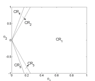
2.13 Critical regions of the mp-DO problem (2.33). . . 55

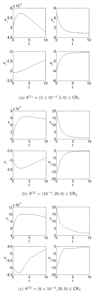
2.14 Selected optimal control and response trajectories of the mp-DO problem (2.33).. . . . 56

2.15 Critical regions of discretized mp-QP counterparts of problem (2.33) forθ3= 0. . . 57

2.16 Closed-loop response of the multi-parametric NCO-tracking controller for problem (2.33). . . 58

3.1 Layer-wise organization of a fully connected neural network . . . 66

3.2 Sample data for training neural network . . . 82

3.3 Trajectory for θ ∈CR₆ _{by mp-DO solution . . . 83}

3.4 Trajectory for θ ∈CR₅ _{by mp-DO solution . . . 84}

3.5 System of two CSTRs operating in series . . . 84

3.6 Optimal solution by mp-DO for CSTRs system in CR₄ _{. . . 89}

3.7 Optimal solution by mp-DO for CSTRs system in CR₈ _{. . . 90}

3.8 Closed-loop response of the mp-NCO-tracking controllers for CSTRs system. 91 4.1 Enclosure of reachability tubes . . . 99

4.2 Interval reachability tubes without K – Case of additive disturbance. . . . 111

4.3 Ellipsoidal reachability tubes without K – Case of additive disturbance. . . 111

4.4 Ellipsoidal reachability tubes – Case of additive disturbance. . . 112

4.5 Critical regions of the mp-DO. Black lines: nominal regions; Blue lines: robust regions. . . 118

(13)

4.6 Robust mp-DO based on ellipsoidal reachability tubes – Case of additive disturbance. . . 119 4.7 Closed-loop performance of the mp-NCO-tracking controllers with ∆T = 1

– Case of additive disturbance. . . 120 4.8 Closed-loop performance of the mp-NCO-tracking controllers with ∆T = 2

– Case of additive disturbance. . . 121 4.9 Comparison on closed-loop performance of the mp-NCO-tracking controllers

– Case of additive disturbance. . . 122 4.10 Ellipsoidal reachability tubes – Case of multiplicative disturbance. . . 123 4.11 Robust mp-DO based on ellipsoidal reachability tubes – Case of

multiplica-tive disturbance. . . 124 4.12 Closed-loop performance of the nominal and robust mp-NCO-tracking

con-trollers – Case of multiplicative disturbance. . . 125 4.13 Nominal solution and worst case enclosure for CSTRs system with additive

disturbance. . . 126 4.14 Robust mp-DO and worst case enclosure for CSTRs system with additive

disturbance. . . 127 4.15 Closed-loop performance of the robust mp-NCO-tracking controllers for

(14)

Chapter 1 Introduction

1.1 Dynamic real-time optimization

On-line optimization and real-time control have received much attention over the past few decades because of the need to improve performance and reduce economic costs in industrial processes [1]. Many such industrial applications involve fast dynamic systems operated under constraints, typically reflecting physical operation bounds and/or safety requirements. To obtain the optimal operation, optimization should be applied to make decisions on the best control action without violating certain constraints. The optimal control action can be obtained by solving optimization problems based on dynamic model of the system involving objective function and constraint functions of state and input variables. An illustrative mathematical representation for dynamic optimization problem considered in this thesis with u(t) as control and x(t) as system states can be written as follows: min u(t),x(t), t₀≤t≤t_f J(x(t), u(t)) s.t. x˙(t) = f(x(t), u(t)) = Fxx(t) +Fuu(t) +f0 g(x(t), u(t)) =Gxx(t) +Guu(t) +g0 ≤0 h(x(tf)) =Hxx(tf) +h0 ≤0 x(t0) =x0, (1.1)

(15)

where t0 and tf are the initial and final times; J(x(t), u(t)) denotes some performance

in-dex that needs to be optimized by choosing the control policy, which is chosen as quadratic objective function J = 1₂x(tf)TQfx(tf) + Rtf t0 1 2x(t)TQx(t) + 1 2u(t)TRu(t)dt with weighting

matrices Qf 0, Q 0, and R ≻ 0; f(x, u) denotes some linear system dynamics with

initial conditionx(t0);g(x(t), u(t)) andh(x(tf)) denotes the path and terminal constraints

for the process which are linear functions of the state and control variables; and all the other notations denote some constant matrices or vectors. The uncertain parameters con-sidered in this thesis lie in linearly in the dynamics, initial conditions and both path and terminal constraints. Besides, robust control is investigated with additive and multiplica-tive disturbances in the linear dynamics f(x(t), u(t)), such that feasibility is guaranteed for all possible scenarios.

A great variety of algorithms have been investigated for solving dynamic optimization problem, which are generally categorized as indirect methods (variational methods) and the direct methods based on discretization. The former transfers the optimization problem into an infinite-dimensional boundary value problem using the corresponding optimality conditions [2, 3]. In the context of direct approach, the catagary includes simultaneous and sequential methods. The simultaneous approach converts the dynamic optimization problem into a finite dimensional nonlinear program by a discretizaiton of both control and state variables, resulting in a set of algebraic qualities and inequalities, where or-thogonal collocation is a popular technique [4–6]. In sequential approach, discretization is achieved via control vector parameterizaiton based on some basis functions that depend on a finite number of decision parameters in the master nonlinear program, which can be subdivided into single shooting and direct multiple shooting methods with continuity constraints for state variables between adjacent time elements [7–9]. The problem with inequality constraints can be solved via either the interior point method [10–12] or sequen-tial quadratic programming [13]. For dynamic optimization, determining global minimum can prove extremely demanding [14] and local optimization techniques are competitive in terms of the computational effort with appropriate variable bounds and good initialization strategies [15].

The standard control scheme in many process industries decomposes a plant’s economic optimization into two layers, the real time optimization (RTO) determines optimal plant operation among all feasible steady-states to minimize the economic objective while

(16)

satis-fying all the constraints [16–18], and the advanced control layer tracks the best set point where model predictive control (MPC) is widely employed [19, 20]. The corresponding hierarchical structure from the planning and scheduling layer to process control layer is shown in Figure 1.1.

process control real time optimization

scheduling planning

Figure 1.1: Illustration of hierarchical operation

The main drawbacks of a two layer control structure include inconsistent models and economics in the dynamic layer, which may lead the set point for steady state to be unreachable for the dynamic layer [16, 21, 22]. Since the control law designed under hierarchical structure usually overlooks the issue of transient costs, the control actions applied to the dynamic systems may be suboptimal by just steering the system to desired state with minimum transition time, yet without considering the economic performance during transient operations. Instead of splitting the control structure into two layers of equilibrium calculation and set point tracking, dynamic RTO (D-RTO) directly optimizes the economic objective to obtain the optimal control actions [23, 24]. The corresponding structure of dynamic RTO is shown in Figure 1.2, where the two-layers are merged into one centralized decision-making layer, and its the synthesis structure can be formulated as economically-oriented MPC.

Dynamic Real-Time Optimization

Real Process

inputs

outputs State & Parameter_Estimation

(17)

A major challenge for process control is the problem of uncertainty stemming from model mismatch and process disturbances where measurement-based method or robust control method needs to be applied. In real applications, uncertainty resulting from model mis-match or disturbances leads the plant to deviate from optimal operation by only imple-menting the nominal control action. Optimization-based methods that repetitively solve for the optimal control should be applied to optimize system performance while satisfying all the constraints. This can be realized by solving the optimal solutions on-line or resort-ing to some novel techniques such as multi-parametric programmresort-ing and NCO-trackresort-ing (tracking the necessary conditions of optimality). The rest of the chapter first presents a brief background on model predictive control and some advanced techniques for re-ducing the on-line computational burdens, including multi-parametric programming and NCO-tracking method. Afterwards, the methodology of the research, multi-parametric NCO-tracking, is introduced alongside a summary of the main contributions, followed by the structure of the thesis.

1.2 Model predictive control

For the current practice in process industry, model predictive control has been widely applied, and the optimal control of industrial plants with stability analysis has reached a solid theoretical foundation [25–27]. Model predictive control, also known as receding horizon control, aims to optimize the system performance in the presence of constraints [16, 28]. It handles the prediction of system dynamic behaviour and constraints at the same time naturally and can accommodate multi-inputs multi-outputs systems as well. Normally, the on-line control implies iteration between parameter estimation and opti-mization problem solving, while in some real applications, the mathematical modelling used for optimization should be updated on-line via parameter estimation. Economic model predictive control is a recently developed technique for optimizing the economic performance of a system subject to operational constraints [16, 17, 29], which falls into the category of dynamic RTO, where dynamic operation is implemented in a receding horizon manner. Classical MPC stability theory usually assumes a cost function that penalizes deviations from a desired steady state to prove stability of the closed-loop system, while in economic MPC, the cost function may not be strictly decreasing along the closed loop trajectory and the average cost is guaranteed to be no worse than that of the best steady

(18)

state under specific periodic state-feedback law [30].

Given the current state of the system, an implicit control law u=κ(x) can be obtained by repetitively solving an optimization problem online as in the form of (1.1) to compute a virtual optimal control sequence in a predictive time horizon ut = [u0, u1, . . . , uN], as

shown in blue dashed lines of input in Figure 1.3 [29, 31]. To compute the optimal control sequence, the dynamic model of the process is used to predict the future dynamic behaviour over a finite time horizon, which might be a couple of minutes or hours, or in infinite time horizon, as shown in blue dashed lines of output in Figure 1.3.

time input time output constraint constraint tk tk+1

Figure 1.3: MPC: virtual optimal input sequence fortk

The cost function to be minimized can be defined in the form:

VN(x, u) = f(xN) + N−1

X

i=0

l(xi, ui)

where f(xN) and l(xi, ui) denote the terminal cost and stage cost, and N denotes the

number of time steps for the finite time horizon.

The optimization problem can be written in the following form: Φ = min u,x VN(x, u) s.t. xi+1 =f(xi, ui) (xi, ui)∈Z ∀i∈I0:N−1 x0 =xt xN ∈XN

where xt denotes the initial condition, which is usually obtained from current state

(19)

state sequence;Z denotes admissible set for the path andXN for the terminal constraints

to guarantee the feasibility of the system.

After the virtual control sequence is obtained, only the first element is applied to the system for the current time interval, i.e. κ(xt) = u0, as shown in blue solid line in

Figure 1.4. time input time output constraint constraint tk tk+1

Figure 1.4: MPC: apply optimal input from tk totk+1

For the next shifted time horizon starting from tk+1,x(tk+1) is taken as the initial

condi-tion, i.e. in the following optimization problem, x0 =x(tk+1), and the new virtual control

sequence is computed as shown in black dashdotted lines in Figure 1.5.

time input time output constraint constraint tk tk+1

Figure 1.5: MPC: new virtual optimal input sequence for tk+1

1.3 Towards off-line computations

The strategy employed in MPC entails the repeated solution of an optimal control problem that predicts the system’s future behaviour over a finite, receding time-horizon, using the current state measurements or estimates as initial conditions [32]. The optimized control

(20)

strategy is implemented until the next measurements become available, and it is the repetition of this process that creates a feedback control. This may prove to be a rather computationally demanding task nonetheless and cause serious delays for fast dynamic systems, thereby leading to performance deterioration or even infeasibility [33, 34]. The computational burden associated to the on-line solution of optimization problems in MPC could be mitigated by solving optimization problems off-line, such as using multi-parametric programming and NCO-tracking, which are introduced in this section. The former method computes the optimal input in an explicit scheme by solving optimization problem off-line [35–37]. For the latter case, instead of solving optimization problem on-line, optimal input is updated directly from system feedback by tracking necessary conditions of optimality corresponding to the optimization problem [38–41].

In the multi-parametric programming paradigm [42–44], solving optimization problem is performed off-line, resulting in an explicit mapping of the control strategies as a function of the initial state of system. For continuous-time systems, this approach gives rise to multi-parametric dynamic optimization (mp-DO) problems, which may either be transformed into finite-dimensional multi-parametric programs via full discretization (direct approach) or handled directly using optimal control theory (indirect approach). In addition, the explicit solution can be applied in MPC, which is referred to as mp-MPC or explicit MPC, and an indicative list of key publications is given in Table 1.1.

Table 1.1: Publications on multi-parametric/explicit model predictive control Multi-parametric MPC Pistikopoulos (1997, 2000), Pistikopoulos and

Morari (2002), Bemporad et al. (2002), Johansen and Grancharova (2003)

Multi-parametric continuous time MPC Kojima and Morari (2004), Sakizlis et al. (2005)

Hybrid multi-parametric MPC Bemporad et al. (2000), Sakizlis et al. (2001, 2003), Borrelli et al. (2005)

Robust multi-parametric MPC Bemporad et al. (2001), Kakalis (2001), Sakizlis et al. (2004), Mayne et al. (2006) Multi-parametric nonlinear MPC Johansen (2002), Bemporad (2003),

Sakizlis et al. (2007), Dominguez and

Pistikopoulos (2010 ,2012), Ziogou et al. (2013)

Besides, a data-driven framework for mp-MPC was proposed based on surrogate modelling and data-classification [45], where the parameter space is divided into regions by using Support Vector Machine [46, 47], and in each region, the first input value of mp-MPC

(21)

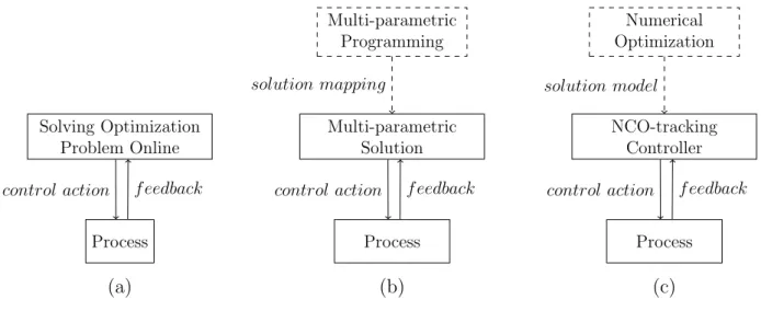
is expressed as an approximate function of states. Thus, the on-line control problem can be computed efficiently by substituting the explicit pre-computed solution mapping for on-line repetitively optimization. Comparison of the closed-loop control profile by directly solving optimization problem on-line and solving off-line using multi-parametric programming is shown in Figure 1.6 (a)(b), where blocks linked with dashed lines denote off-line calculation and blocks linked with solid lines denote on-line updating. The multi-parametric programming approach provides solutions as piecewise affine functions of the parameters, but the resulting solution map usually consists of very large number of critical regions. With the increase on the scale of optimization problems or constraints, the number of critical regions increases significantly.

Process Solving Optimization

Problem Online

control action f eedback

Process Multi-parametric Solution Multi-parametric Programming solution mapping

Process NCO-tracking Controller Numerical Optimization solution model

(a) (b) (c)

Figure 1.6: Comparison between solving on-line and off-line

Another approach to reduce the computational burden in MPC involves tracking the necessary conditions for optimality (NCO), namelyNCO-tracking[40, 48]. In continuous-time, NCO-tracking starts by characterizing the optimal switching structure of the control trajectories. Under the assumption that this switching structure remains unchanged in the presence of uncertainty, feedback laws are then constructed for tracking the active constraints and zero gradient conditions along each arc, and the comparison with on-line optimization is shown in Figure 1.6 (a)(c). A key limitation with the current NCO-tracking methodology nonetheless lies in the fact that the underlying optimal control switching structure might change in the presence of uncertainty; thus, this research aims to close the gap between multi-parametric and NCO-tracking approach for enabling changing switching structures.

(22)

1.4 Contribution and overview

This thesis presents a methodology for combining multi-parametric programming and NCO-tracking into a unified framework, for which we coin the name multi-parametric

NCO-tracking control. By taking advantage of both methods, dynamic real-time

opti-mization is transferred into an on-line tracking problem using feedback controller. Such a combination is especially promising in that multi-parametric programming provides a means for relaxing the fixed switching structure assumption in NCO-tracking, thereby paving the way towards a theoretical justification for NCO-tracking. In addition, the use of feedback laws tracking the optimality conditions inside multi-parametric controller could provide a means for reducing the number of critical regions compared with classical mp-MPC controllers based on control vector parameterization, where the critical region for each multi-parametric switching structure can be regarded as an union of all critical regions in the discrete time case sharing the same switching structures, i.e. the same sequence of active constraints.

In Chapter 2, an algorithm for characterizing the corresponding multi-parametric solu-tion structure in terms of the exact critical regions and nonlinear feedback control laws was proposed for linear-quadratic optimal control problems. A review for both multi-parametric programming and NCO-tracking is first presented in Chapter 2, followed by the detailed presentation of the proposed mp-NCO-tracking control based on the neces-sary conditions of optimality. By solving the mp-DO problem for continuous-time linear dynamic system, the feasible regions, which might be characterized by the initial condi-tions of the systems or some model parameters, are divided into different critical regions. Each region corresponds to an unique control switching structure, i.e. the sequence of arcs, with regard to either active constraints or sensitivity conditions.

The on-line step by using the parametric controller involves determining the critical re-gions containing the measured parameter and applying the corresponding feedback law until next measurement is available. This control framework is readily applied in the receding horizon control. Estimates of states and model parameters can be obtained via on-line estimation approach, enabling the solution structure to be updated by locating the parameter into the corresponding critical region. At the end of the chapter, the framework is illustrated in several case studies for both mp-DO solutions and closed-loop

(23)

simulations, where parameter jumps between different critical regions.

For implementation of mp-NCO-tracking control, a potential difficulty exists in character-ization of the critical regions, where explicit expressions can not be obtained in general. This is due to the fact that the critical regions in mp-DO may be non-convex and closed-form expressions describing their boundaries may not be avaialable in general. Based on fast-developing field of machine learning for classification, data-driven method is applied for the characterization of critical regions in Chapter 3. Among the classification methods in machine learning, neural network is chosen as the model for critical region classification for its ability to represent non-linearities of arbitrary complexity.

The algorithm for training a classifier comprises setting up a neural network model, gener-ating sample data and performing optimization of the network off-line. Once the training process is completed, training data can be completely discarded, and the classifier is em-bedded into the mp-NCO-tracking controllers. The architecture of fully-connected neural network model is presented followed by training the model, where optimization is used for choosing the parameters that characterize the network. Afterwards, an algorithm for the implementation of mp-NCO-tracking is presented, from model set up to trained classifier. Finally, the developments are illustrated by case studies at the end of the Chapter 3. Both classical and multi-parametric MPC controllers are often implemented without con-sidering external disturbances or model mismatch. When large disturbances occur, the constraints can nonetheless become violated, thereby calling for the development of robust control schemes. Thus, a robustification of the mp-NCO-tracking approach is presented in Chapter 4 by extending the multi-parametric controllers for continuous-time linear dy-namic systems subject to bounded uncertainty. The approach involves backing-off the path and terminal constraints based on a worst-case uncertainty propagation, and it is computed based on either interval or ellipsoidal reachability tubes. The uncertain state is decomposed into a nominal reference and a disturbed component, and the effect of disturbance is incorporated into the dynamics of the disturbed component, enclosed by a reachability tube which is centred at the nominal reference trajectory.

A robust-counterpart formulation of the mp-DO problem is formulated considering both additive and multiplicative time-varying uncertainty. Here, the robust formulations retain tractability of the mp-NCO-tracking design problem, thus enabling the direct application

(24)

of the controller design procedure as in the nominal case and making the off-line computa-tional effort independent of the number of uncertain parameters. The result of backing-off the constraints is a modification of the size of the critical regions and possibly the number of critical regions as well—either removing or adding extra regions. The applicability of the approach is demonstrated by case studies for closed-loop simulations.

1.5 Structure of the thesis

The rest of the thesis is organized as follows: Chapter 2 presents the multi-parametric NCO-tracking methodology based on solving the mp-DO problem and the control algo-rithm; Chapter 3 focuses on training a classifier for characterization of critical regions corresponding to the multi-parametric switching structures used for point location em-bedded in the mp-NCO-tracking controller; Chapter 4 develops robust mp-NCO-tracking control based on a robust-counterpart formulation of the mp-DO problem for both addi-tive and multiplicaaddi-tive time-varying uncertainty, considering worst-case scenarios based on set-propagation techniques; Finally, Chapter 5 concludes the thesis and discusses the future directions.

(25)

Chapter 2 Multi-parametric NCO-tracking

control for linear dynamic system

2.1 Introduction

Optimization has played a crucial role in process control over the past years. Optimal control strategies can be determined by solving constrained optimization problems based on a dynamic model of the system. One major challenge with this approach is how to effectively manage uncertainty stemming from model mismatch and process disturbances, as optimal operation needs to be decided on-line using real-time feedback. The strategy employed in classical model predictive control (MPC) [32] handles this uncertainty by repeatedly solving the optimization problem on-line in order to update the optimal inputs. This is often a rather computationally demanding task that may cause serious delays especially for systems with fast dynamics, leading to suboptimal performance or even infeasibility.

In the multi-parametric programming paradigm, the optimization is performed off-line, resulting in a priori explicit mapping of the solutions, effectively control strategies, as a function of measurable quantities [42]. For continuous-time systems, this approach calls for the solution of multi-parametric dynamic optimization problems (mp-DO) [49]. Another approach to reducing the on-line computational burden involves tracking the necessary conditions for optimality, namely NCO-tracking [40, 41, 48]. There, an optimal control policy is obtained indirectly by forcing the NCOs to zero. This process requires

(26)

knowledge of the switching structure of the optimal control, based on which feedback control laws can be derived on account of the available output measurements, effectively converting an optimal control problem into a set of self-optimizing feedback control laws [40, 50]. However, a key assumption for this controller to enable optimal or even feasible operation is that the switching structure should remain unchanged, which may not be the case when large uncertainty is present.

This chapter presents a methodology for combining mp-DO and NCO-tracking into a uni-fied framework for model predictive control, for which we coin the namemulti-parametric

NCO-tracking control. Such a combination is especially promising in that multi-parametric

programming provides a means for relaxing the fixed switching structure assumption in NCO-tracking, while the use of feedback laws by NCO-tracking enables the number of critical regions compared to classical mp-MPC controllers based on control vector param-eterization to be dramatically reduced.

The rest of the chapter is organized as follows. Section 2.2 provides some background for both multi-parametric programming and NCO-tracking method. Section 2.3.2 presents the multi-parametric NCO-tracking methodology, including the use of mp-DO for map-ping subregions of the uncertain parameters to various switching structure and the imple-mentation of the corresponding NCO-tracking controllers in a receding horizon manner. Several numerical examples are given in Section 2.4 to illustrate the approach. Finally, Section 2.5 concludes the paper.

2.2 Background

2.2.1 Review of multi-parametric programming

Multi-parametric (mp) programming is a technology that allows determining the optimal solution as a function of parameters [37], which provides a means for computing the so-lution mapping of an optimization-based control problem off-line based on a model of the dynamic system. The optimal control trajectory is expressed as a function of given param-eters, usually some uncertain measured quantities, thus avoiding the need for repeatedly solving optimization problems on-line when these parameters vary [35–37, 43, 44]. The

(27)

multi-parametric solution calls for the solution of multi-parametric dynamic optimization problems (mp-DO) for continuous-time systems. In practice, such mp-DO can either be transformed into a finite-dimensional multi-parametric program via control vector pa-rameterization [49] or handled directly into its native infinite-dimensional form using the corresponding optimality conditions. In the context of solving the finite-dimensional multi-parametric program, numerous publications exist [35, 37, 42, 51–53], whereas solv-ing the infinite-dimensional counterpart has received relatively little attention [49]. The continuous-time solutions ask for nonlinear critical regions as opposed to its discrete-time counterpart. Thus, the standard techniques for generating linear critical regions can not be applied, and multi-parametric solution can hardly be obtained in general with-out considering the switching structures, which resort to the concept of NCO-tracking. The general theory and algorithms of multi-parametric programming and its applica-tions has been studied in the books [43, 44], and publicaapplica-tions in various algorithms of multi-parametric programming are well summarized in [37, 51]. Overall, the procedure for obtaining multi-parametric solution includes generating critical regions and piecewise affine functions. However, the detailed algorithms may vary based on different types of the optimization problem, which might be linear or nonlinear, with only continuous variables or with integer variables.

Parametric optimal solutions for the infinite-dimensional problem can be obtained by sensitivity analysis, also known as neighbouring extremal (NE) control. In this approach, a feedback law is derived in the neighbourhood of a nominal solution, where the switching structure—namely, the sequence of active path and terminal constraints—remains the same [54–57]; see also [55, 58, 59] for a discussion of the differentiability and stability of parametric solutions. For constrained linear-quadratic optimal control problems in particular, Sakizlis et al. [49] have shown that the mp-DO can be written as a multi-parametric boundary value problem using the Pontryagin Minimum Principle [2, 60, 61]. The continuous-time optimal control trajectory is expressed as a time-varying function of selected parameters, which provides a means for determining the control switching structure using standard multi-parametric programming techniques.

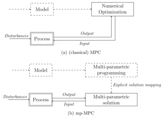
In the context of MPC, multi-parametric programming can be used to obtain the optimal solution of control action as explicit functions of system state feedback or other estimated parameters [37, 42]. A comparison of the control framework of MPC and mp-MPC is

(28)

shown in Fig. 2.1. Instead of repeatedly solving the optimization problem during run-time as in MPC, mp-MPC computes a mapping between the uncertain parameters and their corresponding optimal solutions off-line, and then simply selects the pre-computed control law at run-time after the uncertainty is revealed. The main steps for generating the explicit parametric controller is as follows [42]: develop a high fidelity model of real system and make suitable approximation by system identification or model reduction; design a robust explicit controller; implementation and validation of the designed controller.

Model Numerical Optimization Process Output Input Disturbances (a) (classical) MPC

Model Multi-parametric_programming

Multi-parametric solution

Explicit solution mapping

Process

Output Input Disturbances

(b) mp-MPC

Figure 2.1: Framework of receding horizon control. Dashed lines: off-line task. Solid lines: on-line task.

In the multi-parametric solution based on control vector parameterization, the parameter space is partitioned into a number of critical regions, and the optimal input variable, u, is described by a given function of the parameters, θ, as

u(θ) =                    κ1(θ) if θ ∈CR1, κ2(θ) if θ ∈CR2, ... κn(θ) ifθ ∈CRn. θ1 θ2 CR1 CR2· · · CRn (2.1)

with the critical region illustrated by a two-dimensional parameter space. Here, u(θ) is a finite-dimensional vector that only depends on θ in each critical regions. Each critical

(29)

region corresponds to a unique combination of active constraints and an uniquely defined control law. The boundary of the critical region can be computed from sensitivity analysis of the KKT conditions by keeping the inactive constraints non-binding and the multipliers associated with the active constraints non-negative.

A basic procedure for determining the critical regions is the following [37]:

0. Define the uncertainty domain Θ, and setN = 0. 1. Select a feasible point θ in the region Θ\ ∪N

i=1CRi. If no such point exists, stop;

else, set N ←N+ 1.

2. Construct the critical region CRN aroundθ, wherein the active constraints are the

same, e.g. using sensitivity analysis of the KKT conditions. 3. Return to step 1.

4. Unify the regions and solutions for a more compact representation.

On termination, this procedure returns the number N of critical regions contained in the initial domain Θ. In step 2 for the critical region construction, let ˇg(u, θ) denote inactive constraints and ˆλ(u, θ) denotes the Lagrangian associated with active constraints; then the critical regions including the feasible point selected can be defined as:

CRN:=      ˇ g(u, θ)≤0 ˆ λ(u, θ)≥0

For linear problems involving parametric linear programming (mp-LP) and multi-parametric quadratic programming (mp-QP), there exist exact solutions [35], and details about formulating the problems can be found in [62]. The main result of multi-parametric programming is the solution mapping of the control problem, where the input can be expressed as a linear function of parameters u=a1θ+a0. A linear mp-MPC problem is

presented later in the following paragraphs to illustrate the procedure based on solving a mp-QP problem (2.3). The same example is used throughout the theoretical part of this chapter to illustrate the developments.

(30)

Illustrative example We consider the problem to steer the state x(t) of the following second-order system to zero, by manipulating the bounded input u(t)∈[−2,2]:

˙ x(t) =  −3 −2 1 0   | {z } Fx x(t) +  1 0   |{z} Fu u(t). (2.2)

The mp-MPC problem obtained by discretizing the dynamics on N time intervals along the time horizon 0 ≤t≤1 reads

min u,x x T NQfxN + 1 N N−1 X k=0 xT_kQxk+u2k (2.3) s.t. xk+1 =Fxxk+Fuuk, k= 0. . . N−1 −2≤uk ≤2, k= 0. . . N−1 x0 =θ,

where the parameters θ ∈ [−2,2]2 _{corresponds to the initial state; the matrices} _F x and

Fu in the discretized system are given by

Fx = exp (FxT) and Fu = Z T 0 exp (Fx(T −t))dt Fu,

with the sampling time T := 1/N; and the weighting used in the objective function is as follows Qf =  0.8198 0.8198 0.8198 10.82  , Q=  10 0 0 10  , and R = 0.1.

Numerical solution of the mp-QP (2.3), here using the PAROC framework [52], provides expressions of the optimal controls u = [u0, . . . , uN−1] as explicit functions of the initial

conditions θ, in the form (2.1). The critical regions for the optimal solution are shown in Fig. 2.2(a) in the caseN = 10, whereby each region CRi corresponds to a piecewise affine

functions u = Kiθ+ki, with Ki ∈ RN×2 and ki ∈ RN. Here, the region labelled CR08

in the central part corresponds to the case that none of the input constraints are active. The regions aboveCR08_{correspond to the input lower bound being active for one or more}

(31)

increases. Likewise, the regions below CR08 _{correspond to the input upper bound being}

active for one or more time intervals.

(a) N= 10

(b) N = 20

Figure 2.2: Critical regions for the mp-QP (2.3).

For comparison, critical regions in the case N = 20 are shown in Fig. 2.2(b). Here again, the region in the center corresponds to unconstrained solution and other regions, either above or below it, correspond to input constraints being active for the first few time intervals. The multi-parametric solution becomes more accurate due to the use of a smaller sampling time, but at the same time the number of critical regions increases significantly, thereby defining a trade-off between accuracy and computational tractability. In contrast, the approach proposed in this paper removes the need for discretizing the dynamics and the control trajectories, in order to reduce the number of critical regions.

(32)

2.2.2 Review of NCO-tracking

NCO-tracking is a measurement-based optimization approach to enforce optimality in the presence of uncertainty via tracking of the necessary conditions for optimality (NCO) [40, 63]. This way, a dynamic optimization problem is transformed into a feedback control problem, which may lead to a large reduction of the on-line computational effort by avoiding the repeated solution of an optimal control problem.

The design of the NCO-tracking controllers starts by detecting the switching structure of the optimal control in order to formulate a feedback strategy via appropriate pair-ing between the input and output variables—the so-called solution model [39, 41], see Fig. 2.5(a). In the feedback loop, input is updated directly by enforcing the system to meet the corresponding necessary conditions in solution model. A specific switching struc-ture is characterized by a unique sequence of arcs and the solution model involves the types of each arc and the switching times [39], which normally comes from the concept of minimum principle. For the solution of a dynamic optimization problem, the optimal trajectory corresponds to a unique sequence of active path constraints and active terminal constraints, which can be characterized by solving the first-order NCO for the problem. More details can be found in [2, 39, 64], and the corresponding equations of optimal conditions for the dynamic optimization problem considered in this thesis consists of (2.6) -(2.19) in section 2.3.2.1.

An illustration of a sequence of arcs and switching times in solution structure can be found in Figure 2.3, where u1, u2, u3 denote different arcs that specific optimal conditions

need to be satisfied between time intervals defined by switching timest1, t2. The switching

times as well as the parameters in parameterized input profiles are the decision variables to be adjusted through NCO-tracking.

Along each arc, a certain combination of inputs may be used for tracking the active path constraints, whereas the remaining inputs are adapted for forcing stationary conditions (gradients) to zero. This latter forcing usually calls for approximation techniques, such as neighboring-extremal control [38, 65–67] or extremum-seeking control [68, 69]. The sen-sitivities of the control variables with respect to the uncertain parameters are obtained through variation of the first-order NCO at the nominal solution [70, 71]. For singular problems, by the singular value decomposition to split input profiles into nonsingular and

(33)

t u u1 u2 u3 t0 t1 t2 tf

Figure 2.3: A switching structure with three arcs

singular parts, the latter can be determined form additional differentiation [72]. Combin-ing NCO-trackCombin-ing and self-optimizCombin-ing together is discussed in [73], where both represent first-order approximations to the classical two-step approach of RTO [74]. It is sometimes possible to arrive at a fully decentralized control scheme, for instance using directional information [40, 50, 75]. In order to steer process to the optimal operation, the online feedback controller requires reliable estimates of NCO parts which are possible for path constraints but not for terminal constraints or sensitivity arc, where model based predic-tion is needed for making decision.

It may be noted that the sequence of arcs in solution model actually contains the same information as the critical region in the context of multi-parametric programming. The unique combination of active constraints in multi-parametric programming also corre-sponds to a sequence of active constraints in the time domain, which can be considered as a certain switching structure with several arcs.

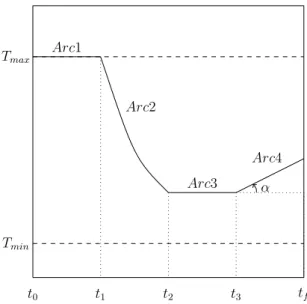
An example of emulsion copolymerization of styrene/α-methylstyrene in a batch reactor [50] is presented here to explain the solution structure as a sequence of arcs. The reactor temperatureT(t) is manipulated to minimize the batch time while satisfying the bounded constraints on reactor and jacket inlet temperature as well as some performance demand.

(34)

The optimization problem based on the dynamic model in [76] for this case is as follows min T(t),tf tf s.t. x˙(t) = f(x(t), u(t)) x(0) =x0 Tmin ≤T(t)≤Tmax

Tjinmin ≤Tjin(t) X(tf)≥Xfd Mn(tf)≥Mnfd

where the first constraint is the tendency model for the process, including state variables like monomer concentration and reactor and jacket temperature. The following constraints correspond to bounds on the reactor temperature, the jacket inlet temperature, the final conversion and number average molecular weight, respectively. The optimal operation of reactor temperature, as shown in Figure 2.4, consists of a sequence of four arcs, each cor-responds to some active constrains or sensitivities conditions: arc 1 – reactor temperature is maintained at its maximal value Tmax to accelerate the nucleation, i.e. the third

con-straint of its upper bound is active; arc 2 – reactor temperature takes value betweenTmax

and Tmin to avoid shorter polymer chains and lower molecular weights by imposing lowest

jacket inlet temperature Tjinmin, i.e. the four constraint on its lower bound is active; arc

3 – temperature is maintained at some optimal constant value, for any increase will lead to smaller average molecular weight; finally arc 4 – the last step without monomer supply and the reactor temperature should be increased to compensate for a drop in reaction rate with the increasing slope α as a decision variable, with the initial temperature fixed at the temperature of arc 3. Besides, the two terminal constraints are forced to be active for the batch to be optimal. In total, there are three jumps between arcs at switching times t1, t2 and t3, where optimal control policy switches to meet the specific operating

conditions corresponding to each arc.

A key limitation with the current NCO-tracking methodology nonetheless lies in the fact that the underlying optimal control switching structure is known in advance and assumed to keep unchanged, but it might change in the presence of uncertainty. As a result, the NCO-tracking controller may be suboptimal and could even lead to infeasible operation due to constraint violation. Although the assumption of a constant structure is often

(35)

Tmin Tmax t0 Arc1 t1 Arc2 t2 Arc3 t3 Arc4 α tf

Figure 2.4: Nominal optimal reactor temperature profile

satisfied in batch process optimization applications [77], it is not well suited for MPC applications where constraints frequently activate or deactivate.

It has been suggested that the control switching structure could be monitored by some supervisory system [38]. The developments in this chapter provide the foundations for such an approach to handling a varying optimal switching structure, such that process operation remains feasible and optimal. The operation relies on the mapping between uncertain parameters and optimal switching structures using mp-DO, and the subsequent formulation of optimal control laws that can be applied in a receding horizon manner, namely multi-parametric NCO-tracking controllers.

2.3 Methodology for multi-parametric NCO-tracking

control

2.3.1 Problem statement

The main contribution of this chapter is a methodology for the derivation of multi-parametric NCO-tracking controllers for constrained linear-quadratic optimal control

(36)

prob-Model _OptimizationNumerical NCO-tracking Controller Solution Model Process Output Input Disturbances

(a) classical NCO-tracking

Model Multi-parametric Dynamic Optimization Multi-parametric NCO-tracking Controller Critical Regions Process Output Input Disturbances (b) multi-parametric NCO-tracking

Figure 2.5: Principle of NCO-tracking methodology lem in the form:

Φ(θ) := min u(t),x(t), t₀≤t≤t_f 1 2x(tf) T_Q fx(tf) + Z tf t0 1 2x(t) T_Qx₍_t_{) +} 1 2u(t) T_Ru₍_t₎_dt s.t. x˙(t) = f(x(t), u(t)) :=Fxx(t) +Fuu(t) +Fθθ+f0 g(x(t), u(t)) :=Gxx(t) +Guu(t) +Gθθ+g0 ≤0 h(x(tf)) :=Hxx(tf) +Hθθ+h0 ≤0 x(t0) = Bθθ+b0, (2.4)

where Φ is the optimal value function; x(t)∈ Rnx _and _u₍_t₎_∈_Rnu _{are the state variables}

and input variables, respectively, at a given time t; t0 and tf are the initial and final

times; g :Rnx _×_Rnu _→ _Rng _and _h _:_Rnx _→ _Rnh define the path and terminal inequality

constraints; and Qf 0, Q 0, and R ≻ 0 are given weighting matrices. We assume

that the uncertain parametersθ ∈Rnθ appear linearly in the initial conditions, dynamics,

path constraints, and terminal constraints of problem (2.4).

The proposed methodology involves two steps, as depicted in Fig. 2.5(b):

• The first (off-line) step defines the multi-parametric control structure, namely map-ping the optimal control structure to given measurable quantities, such as the uncer-tain initial conditions, using mp-DO. This results in a partitioning of the unceruncer-tain

(37)

parameter domain into a number of critical regions, each corresponding to a unique sequence of active path constraints and active terminal constraints. As well as giv-ing a set of conditions for characterizgiv-ing each critical region, mp-DO determines feedback control laws in the form:

u(t) = K(i)_{t, θ, t}(i)

1 (θ), . . . , t (i) Nt(i)

(θ) , (2.5)

where the junction times t(₁i)(·), . . . , t(i)

Nt(i)

(·) in the optimal switching structure for critical region CRi are themselves dependent onθ.

• In the subsequent (on-line) step, the multi-parametric NCO-tracking controller is applied in a receding horizon manner. This involves determining the critical regions containing the measured parametersθ and applying the corresponding feedback law until a new measurement becomes available at the next sampling time. Because the switching time functions t(_ki)(·) are typically defined implicitly in practice, even for constrained linear-quadratic control problems, one can either derive fully explicit feedback laws by approximating this functional dependency, or else apply a Newton iteration to compute the t(_ki) for given values of θ at each sampling time.

Both steps are detailed subsequently.

Notation Dα

xf denotes theα-th partial derivative of a functionf with respect toxand

f(j)_{, the} _j_{-th order derivative of with respect to} _t_{. The path constraint} _g

i is said to be of

order (or degree) σi ≥0 if Dug(ij) ≡0 for j = 0. . . σi−1 andDugi(σi) 6= 0, or equivalently,

Gx,iFxσi−1Fu 6= 0 and Gu,i =Gx,iFxFu =· · ·=Gx,iFxFσi−2Fu = 0.

For simplicity, we introduce the notation

g_i(j)(x, u) := G_x,i(j)x+G_u,i(j)x+G(_θ,ij)θ+g(₀j_,i),

where the row vector G(_x,ij), G(_u,ij), G_θ,i(j) and scalar g₀(j_,i) can be expressed in terms of Fx, Fu,

Fθ,fθ, Gx,Gu, Gθ and g0, for each j = 1. . . σi. We also make use of the notation

(38)

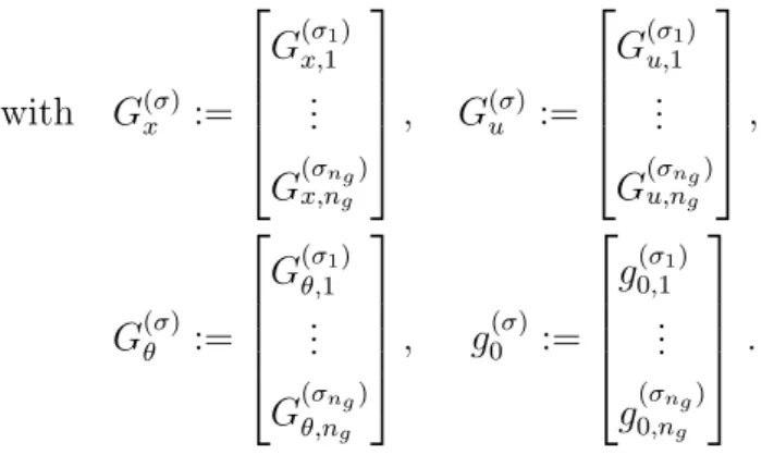
with G(_xσ) :=      G(σ1) x,1 ... G(σng) x,ng      , G(_uσ) :=      G(σ1) u,1 ... G(σng) u,ng      , G(_θσ) :=      G(σ1) θ,1 ... G(σng) θ,ng      , g₀(σ) :=      g(σ1) 0,1 ... g(σng) 0,ng      .

Finally, by a slight abuse of the notation, an over-bar is used to indicate subsets of the terminal or path constraints that are active along a given arc, such as ¯g(x(t), u(t)) =

¯

Gxx(t) + ¯Guu(t) + ¯Gθθ+ ¯g0 ≤0 and ¯µ(t).

Besides, a list of the notations used for developing multi-parametric solutions in the following sections can be found in Table 2.1.

Table 2.1: List of notations

x(t) continuous-time state variable

u(t) continuous-time control variable

p(t) continuous-time co-state variable

S switching structure

Nt the number of arcs

tk switching times

µ(t) multipliers for path constraint

ν multipliers for terminal constrains

H Hamiltonian function

π multipliers at points of discontinuity of p(t) ACk sets of active path constraints along the kth arc

NACk sets of inactive path constraints along the kth arc

ACf sets of active terminal constraints

NACf sets of inactive terminal constraints

ENk sets of path constraints activating at tk

EXk sets of path constraints deactivating at tk

COk sets of path constraints contacting at tk

2.3.2 Multi-parametric dynamic optimization

2.3.2.1 Solution structure

For each instance of the parameters θ, the optimal solution of problem (2.4) exhibits a certain switching structure, denoted by S(θ). The sequence of active path constraints and active terminal constraints can be characterized by solving the first-order NCO for

(39)

Problem (2.4), which come in the form of a multi-point boundary value problem [2]. Under the assumption that the number of arcs Nt(θ) is finite for each parameter value [78], we

denote by tk(θ), k = 1. . . Nt−1(θ), the sequence of junction times for each arc in S(θ),

with t0(θ) = t0 and tNt(θ) =tf. These times correspond to the activation or deactivation

a particular path constraint or to a touch-and-go point for a higher order path constraint. We denote the sets of path constraints activating, deactivating, or contacting at tk(θ) by

ENk(θ), EXk(θ) and COk(θ), respectively. Moreover, ACk(θ) and NACk(θ) denote the

sets of active/inactive path constraints along thekth arc,t+_k₋₁(θ)≤t≤t−

k(θ); and ACf(θ)

and NACf(θ), the sets of active/inactive terminal constraints.

Besides its switching structure, characterizing an optimal solution involves determining: (i) the quadruplet of trajectories (u(t), x(t), p(t), µ(t)) along each arc, wherep(t)∈Rnx _are

the co-state (adjoint) variables, and µ(t) ∈Rng_{, the multipliers for the path constraints;}

(ii) the values of the multipliers ν ∈Rnh for the terminal constraints; and (iii) the values

for the multipliers π_k,ij for j = 1. . . σi −1, i = 1. . . ng, k = 1. . . Nt(θ)−1 at points of

discontinuity of the co-state trajectories p(t) (if any). Provided certain controllability and regularity assumptions hold (see below), the following conditions must be satisfied at an optimal solution of Problem (2.4), according to the indirect adjoining approach [61]:

(i) Along each arc t+_k₋₁(θ)≤t ≤t−

k(θ), fork = 1. . . Nt(θ): ˙ x(t) = ∂H ∂p(u(t), x(t), p(t), µ(t)) = Fxx(t) +Fuu(t) +Fθθ+f0 (2.6) ˙ p(t) =−∂H ∂x(u(t), x(t), p(t), µ(t)) =−Qx(t)−F T xp(t)−G(xσ) T µ(t) (2.7) 0 = ∂H ∂u(u(t), x(t), p(t), µ(t)) =Ru(t) +F T up(t) +G(uσ) T µ(t) (2.8)

0 =µi(t)gi(x(t), u(t)) =µi(t) (Gx,ix(t) +Gu,iu(t) +Gθ,iθ+g0,i) (2.9)

(−1)jµ(_ij)(t)≥0≥gi(x(t), u(t)) =Gx,ix(t) +Gu,iu(t) +Gθ,iθ+g0,i, (2.10)

for each i= 1. . . ng and eachj = 1. . . σi, and with the Hamiltonian function

H(u, x, p, µ) := 1 2x T_Qx₊1 2u T_Ru₊_pT₍_F xx+Fuu+Fθθ+f0) +µT_G(σ) x x+G(uσ)u+G (σ) θ θ+g (σ) 0 . (2.11)

(40)

(ii) At the terminal time tf =tNt(θ)(θ):

p(tf) = Qfx(tf) +HxTν (2.12)

0 =νihi(x(tf)) =νi(Hx,ix(tf) +Hθ,iθ+h0,i) (2.13)

νi ≥0≥hi(x(tf)) =Hx,ix(tf) +Hθ,iθ+h0,i, (2.14)

for each i= 1. . . nh.

(iii) At each junction timetk(θ), fork = 1. . . Nt(θ)−1:

H(u(t− k), x(tk), p(t−k), µ(t − k)) = H(u(t + k), x(tk), p(t+k), µ(t + k)) (2.15) p(t− k) = p(t + k) + ng X i=1 σi X j=1 πj_k,iDxgi(j)(x(tk), u(t+_k)) =p(t+_k) + ng X i=1 σi X j=1 π_k,ij G(_x,ij) (2.16) 0 =π_k,ij gi(x(tk), u(t+k)) (2.17) πj_k,i              ≥(−1)σi−1µ(σi−1) i (t+k), if i∈ENk(θ)∪COk(θ) and j = 1 = (−1)σi−jµ(σi−j) i (t+k), if i∈ENk(θ) and j >1 = 0 otherwise (2.18) µ(σi−j) i (t − k) = 0, if i∈EXk(θ)∪COk(θ) and 0≤j ≤σi−2, (2.19)

for each i= 1. . . ng and eachj = 1. . . σi.

Note that the multipliers π may only appear in the optimal conditions for problems with pure state path constraints of order 1 or higher; they can be discarded in problems having mixed control-state path constraints only, where the adjoint trajectories are continuous at junction times.

In general, the foregoing optimality conditions (2.6)-(2.19) are only necessary under the additional assumptions that: (i) the pair (Fx, Fu) is controllable, which precludes

ab-normality [79]; and (ii) both the active path and active terminal constraints are regular [61], rankh_G¯(σ) u g(x(t), u(t)) i = ng, t+_k₋₁(θ)≤t≤t−_k(θ), k= 1. . . Nt(θ), and rankhHx h(x(tf)) i = nh.

(41)

Moreover, under the extra assumption of strict complementarity slackness for the multi-pliers ν, π_k,ij and µ(t) along each arc t+_k₋₁(θ0) ≤ t ≤ t−_k(θ0) for a given parameter value

θ0, and by strict convexity of the objective function and linearity of the dynamics and

constraints, the optimal trajectories u(t), x(t), p(t), µ(t) for t+_k₋₁(θ0) ≤t ≤t−_k(θ0),

opti-mal multipliers ν and πj_k,i, and optimal switching/contact times tk describe differentiable

functions in an (open) neighborhood of θ0 [57–59]; see also [49]. Expressions for these

functions are established in the following subsection.

2.3.2.2 Feedback control laws

Using the previous optimality conditions, explicit feedback control laws can be derived along each arc of the optimal solution. Using condition (2.8), together with the fact that ¯

g(σ)₍_x₍_t₎_{, u}₍_t_{)) = ¯}_G(σ)

x x(t) + ¯G(uσ)u(t) + ¯G(_θσ)θ+ ¯g0(σ) = 0 along an arc, we have

¯ µ(t) = hG¯(_uσ)R−1 G¯(_uσ)Ti−1hG¯(_xσ)x(t)−G¯(_uσ)R−1FT up(t) + ¯G (σ) θ θ+ ¯g (σ) 0 i (2.20) u(t) = −R−1hFT up(t) + ¯G(uσ) T ¯ µ(t)i (2.21)

which are both well-defined under the assumption that ¯G(uσ) is full rank. In turn, the state

and co-state equations (2.6)-(2.7) can be rewritten in the form

 x˙(t) ˙ p(t)  =  Φ (k) xx Φ(xpk) Φ(pxk) Φ(ppk)   | {z } A(_xpk)  x(t) p(t)  +  Φ (k) xθ Φ(_pθk)   | {z } A(_θk) θ+  ϕ (k) x0 ϕ(_pk₀)   | {z } a(₀k) (2.22) with: Φ(_xxk) :=Fx−FuR−1 G¯(uσ) Th_¯ G_u(σ)R−1 G¯_u(σ)Ti−1G¯(_xσ) Φ(_xpk) := − Fu−FuR−1 G¯(uσ) Th_¯ G_u(σ)R−1 G¯_u(σ)Ti−1G¯(_uσ) R−1FT u Φ(_xθk) :=Fθ−FuR−1G¯(uσ) Th_¯ G_u(σ)R−1 G¯_u(σ)Ti−1G¯(_θσ) ϕ(xk0) :=f0−FuR−1 G¯(uσ) Th_¯ G_u(σ)R−1 G¯_u(σ)Ti−1g¯0(σ) Φ_px(k) := −Q− G¯(_xσ)ThG¯_u(σ)R−1 G¯(_uσ)Ti−1G¯(_xσ) Φ(_ppk) := −Φ(_xxk) Φ(_pθk) := − G¯(xσ) Th_¯ G(uσ)R−1 G¯(uσ) Ti−1 _¯ G(_θσ)

(42)

ϕ_p(k₀) := − G¯_x(σ)ThG¯_u(σ)R−1 G¯(_uσ)Ti−1g¯(₀σ).

This way, we may express x(t) and p(t) at each t ∈ [t+_k₋₁(θ), tk(θ)−], and therefore also

u(t) and µ(t), as parametric functions of the uncertainty θ, the junction timestk, and the

state/co-state values at tk:  x(t) p(t)  = exp A(_xpk)[t−tk−1(θ)]  x(tk−1(θ)) p(t+_k₋₁(θ))  + Z t tk−1(θ) exp A(_xpk)[t−τ] hA_θ(k)θ+a(_θk)i dτ . (2.23)

In the case that A(xpk) is nonsingular, we have:

 x(t) p(t)  = exp A(_xpk)[t−t_k₋₁(θ)]    x(tk−1(θ)) p(t+_k₋₁(θ))  + A(_xpk)−1 h A(_θk)θ+a(_θk)i   − A(_xpk)−1 hA_θ(k)θ+a(_θk)i . (2.24)

When A(xpk) is singular, an explicit expression can be obtained by considering the normal

Jordan form of A(xpk) instead.

At this point, parametric expressions for the terminal and interior-point constraint mul-tipliers ν and πk can be obtained by piecing together (2.23) on [t0, tf] and exploiting the

equality conditions in (2.12)-(2.13) and (2.16)-(2.19). In the case of mixed state-input path constraints only, the optimal state and co-state trajectories are both continuous at the junction times. Then, since ¯Hx is full rank, and provided that A(xpk) is invertible on

each arc, parametric expressions for the active terminal constraint multipliers ¯ν, terminal state x(tf) and initial adjoint p(t0) can be obtained from the following linear system:

0 = ¯Hxx(tf) + ¯Hθθ+ ¯h0 (2.25)   x(tf) Qfx(tf) + ¯HxTν¯  = exp   Nt(θ) X k=1 A(_xpk)[tk(θ)−tk−1(θ)]    Bθθ+b0 p(t0)   (2.26) + Nt(θ) X k=1 exp   Nt(θ) X j=k+1 A(_xpj)[tj(θ)−tj−1(θ)]   exp A(_xpk)[tk(θ)−tk−1(θ)] −I A(_xpk)−1hA_θ(k)θ+a(₀k)i.

(In the case of a single control arc, Nt(θ) = 1, the term PjN=t(kθ+1) A (j)

(43)

right-hand side of (2.26) cancels to zero.)

Overall, for a given structureS(θ), the solution of Problem (2.4) can therefore be expressed in parametric form as

(u(t), x(t), p(t), µ(t), ν, π) = FS(θ) t, θ, t1(θ), . . . , tNt(θ)−1(θ)

. (2.27)

Naturally, this construction can be automated in a practical implementation. One could also exploit the remaining optimality conditions (2.15) in order to determine parametric expressions of the junction times tk as a function of θ alone. Explicit expressions are

often not possible, however, due to the inherent nonlinearity of the parametric state/co-state expressions (2.23) in tk and θ. In practice, one may either use approximate explicit

expressions for tk(θ), or compute these junction times on-line using a Newton iteration.

These considerations are discussed further in Section 2.3.3.

2.3.2.3 Critical regions

Each critical region corresponds to a subset of the uncertain parameter domain Θ⊆Rnθ_,

whereby the corresponding optimal control solutions all share the same switching struc-ture in terms of the sequence of active path constraints and active terminal constraints. Formally, given the switching structureS comprised of Nt arcs with corresponding index

sets ENk, EXk, COk, ACk, NACk, ACf, and NACf, the critical region CRS associated

with S is defined as CRS :=                                              θ ∈Θ ∃x(·), u(·), p(·), µ(·), ν, π, t1, . . . , tNt−1 : (u(t), x(t), p(t), µ(t), ν, π) =FS(t, θ, t1, . . . , tNt−1) t0 ≤t1 ≤ · · · ≤tNt−1 ≤tf H(u(t−_k), x(tk), p(t−k), µ(t − k)) =H(u(t+k), x(tk), p(t+k), µ(t+k)), k = 1. . . Nt−1 (−1)j_µ(j) i (t)≥0, i∈ACk, t∈[t+k−1, t − k], k= 1. . . Nt gj(x(t), u(t))≤0, j ∈NACk, t∈[t+k−1, t − k], k= 1. . . Nt π1 k,i≥(−1)σi−1µ (σi−1) i (t+k) ifσi >0, i∈ENk∪COk, k= 1. . . Nt−1 νi ≥0, i∈ACf hj(x(tf))≤0, j ∈NACf                                              (2.28)